Introduction
Setting up your environment properly can save hours of debugging later.
In this guide, we’ll walk through how to configure VS Code and Anaconda for efficient data analysis and visualization, from installing essential tools to connecting with databases.
Required Tools
- Anaconda — For managing Python environments and packages
- VS Code — As the main code editor
- DBeaver — For managing databases visually
- Git / GitHub — For version control
Ensure all required tools above are installed and properly configured.
Optional Tools
- Mamba — Faster alternative to Conda
- Docker — For containerized setups
- GitHub CLI — For managing GitHub directly from your terminal
VS Code Extension
| Extension | Purpose | |
|---|
| Python | Core support for Python syntax, debugging, and linting | |
| Jupyter | Run notebooks directly inside VS Code | |
| Pylance | Provides fast, intelligent code completion | |
| GitLens | Adds advanced Git insights | |
| Database | Helps connect and query databases within VS Code | |
| Data Wrangler | Lets you explore and clean data directly in VS Code | |
| Remote - SSH / Dev Containers (optional) | Work inside containers or remote servers | |
| NOTE | | |
DBeaver is not a database replacement; it’s a universal database management tool. Here’s why developers and data engineers prefer it:
- Multi-database Support
- Friendly User Interface
- Advanced Features
- Cross-platform
Anaconda
In Anaconda, you’ll create an environment. Think of an environment as a separate workspace or bubble for a specific project.
Inside that bubble, the environment can have:
Its own version of Python.
Its own installed package.
Its own settings.
- Command to create an environment
conda create -n <your_environment_name> python=3.10
Replace <your_environment_name> with the actual name of the environment you want to create
- Activate the environment you just created
conda activate <your_environment_name>
Replace <your_environment_name> _with the actual name of the environment you want to create
Once your environment is activated, you’ll notice its name appear in parentheses at the beginning of your terminal prompt.
This means that you’re now working inside that specific Conda environment, and any commands you run or packages you install will apply only to it.
- Install Essential packages
Now that we’ve created and activated our Conda environment, the next step is to install the essential Python packages we’ll use for data analysis and visualization.
These packages provide powerful tools for working with data, building visualizations, connecting to databases, and managing our Jupyter environment.
Core Libraries
- pandas — For data manipulation and analysis
- numpy — For numerical computations
- seaborn & matplotlib — For data visualization
- sqlalchemy — For database connections and queries
- python-dotenv — For managing environment variables
- ipykernel — To link this environment with Jupyter
- jupyterlab / notebook — For interactive data exploration
Database Drivers
If you’ll be working with different database systems, you’ll need the appropriate drivers to connect to them:
- psycopg2-binary → PostgreSQL
- pymysql → MySQL
- pyodbc → SQL Server
Machine Learning & Utilities
To extend your data workflow, it’s helpful to include some additional tools:
- scikit-learn — For machine learning and modelling
- nbstripout, pre-commit — For cleaning notebooks and maintaining project hygiene
- plotly — For interactive visualisations
- pyarrow — For working with large datasets and file formats like Parquet
- Installation commands
With your conda environment active, run the following command to install the main set of libraries:
conda install pandas numpy seaborn matplotlib sqlalchemy python-dotenv ipykernel jupyterlab scikit-learn plotly pyarrow -y
Then, install the database drivers and project utilities using pip:
pip install psycopg2-binary pymysql pyodbc nbstripout pre-commit
- Bonus: Register the Environment in Jupyter
Once all installations are complete, ensure that your new Conda environment is available as a kernel in Jupyter. Run:
python -m ipykernel install --user --name <your_enviroment_name> --display-name "Data Analysis Env"
Replace <your_environment_name> _with the actual name of the environment you want to create
This allows you to select your environment directly from JupyterLab or Notebook.
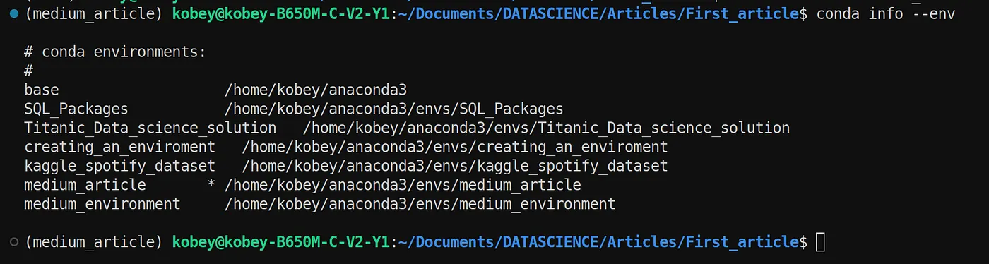
At this point, you can list all your Conda environments using the following command. The environment marked with an asterisk (*) is the one currently active.
conda info --env
Git and Repository Hygiene
With your environment ready, it’s time to set up version control and project hygiene tools.
These tools help you maintain clean, organised repositories, especially when collaborating or working with large datasets and notebooks.
Ensure you have Git installed and configured with your GitHub account.
Git and GitHub setup
Make sure you’re inside your project folder:
cd <your-project-directory>
Create your first notebook in the root folder:\
touch first_notebook.ipynb
Then initialize Git:
git init
This creates a hidden .git folder; your project is now under version control.
Add your project files
git add .
Then commit them
git commit -m "Initial commit"
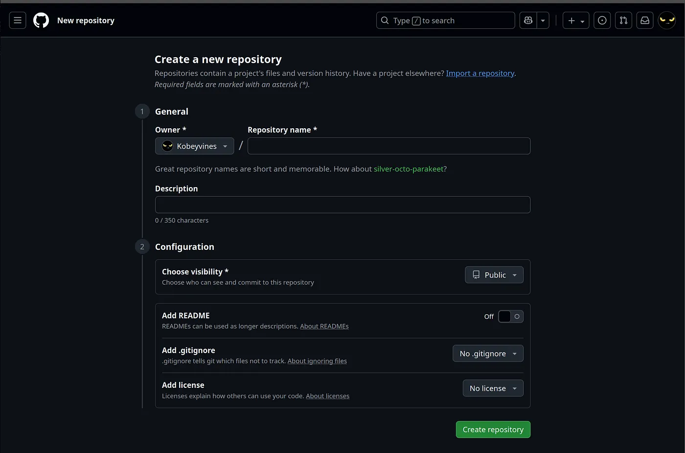
**Create a new repository on GitHub
- Go to https://github.com/new
- Name it something like data_env_setup or whatever matches your project.
- Leave “Initialise with README” unchecked (you already have files locally).
- Click Create repository.
Connect local repo to GitHub
GitHub will show you a few commands after creating the repo; use the HTTPS version, and copy the URL provided:
In your terminal, run:
git remote add origin <paste the url you copied from github>
Example in my case:
git remote add origin https://github.com/Kobeyvines/data_env_setup.git
Push your initial code structure to GitHub:
git branch -M main
git push -u origin main
Git LFS(Large File Storage)
Data projects often involve large datasets, models, or binary files that shouldn’t be stored directly in Git.
Git LFS (Large File Storage) solves this by storing large files outside your main Git history and replacing them with lightweight text pointers.
This keeps your repository fast, clean, and efficient.
Install:
sudo apt update && sudo apt install git-lfs -y
Initialise Git LFS:
git lfs install
Track Large Files
To tell Git LFS which file types to handle, run:
git lfs track "*.csv"
git lfs track "*.parquet"
git lfs track "*.pkl"
Then commit the changes:
git add .gitattributes
git commit -m "Configure Git LFS for large files"
This creates or updates a .gitattributes file in your project root, Git uses this file to know which files should be managed by LFS.
Note: We are saving our data tracking specifically for DVC next, keeping Git LFS reserved strictly for non-data engineering assets like model binaries.
Structure Your Project and Add Your Dataset
As data workflows grow, keeping datasets loose in the root folder gets messy. It’s best practice to organize your data into a dedicated directory. Let’s create a data/ folder and place our dataset inside it.
Your project structure should look like this:
First_article/
├── data/
│   └── 01-raw
|	└── 02-preprocessed
|	└── 03-features
|	└── 04-predictions
├── notebooks/
│   └── EDA.ipynb
├── .git/
├── .gitignore
└── .gitattributes
DVC (Data Version Control)
When working on data science or machine learning projects, version control goes beyond just tracking your code. You also need to manage datasets, pipeline steps, and large data folders that change constantly.
That’s where DVC (Data Version Control) comes in. DVC extends Git to handle data the same way Git handles code, allowing you to version control entire directories without bloating your Git history.
Install DVC:
pip install dvc
Initialize it in your project:
Run the following in your project’s root directory:
dvc init
This command sets up a .dvc/ folder that stores configuration and cache tracking files. Think of it as DVC’s control center.
(Optional but Recommended) Enable Auto-Staging:
Before we add our data, let’s simplify our workflow by enabling DVC’s auto-staging feature:
dvc config core.autostage true
This tells DVC to automatically stage any generated .dvc and .gitignore files for Git whenever you track data, saving you from running repetitive git add commands manually.
Add and Track Your Data Folder
Instead of tracking individual CSV files one by one, we will track the entire data/ directory. This scales beautifully as you add raw, processed, or validated datasets to your project.
Run the following command:
dvc add data
What just happened?
- DVC created a
data.dvc file in your root directory. This is a lightweight text pointer containing a unique hash (checksum) of your data folder.
- DVC automatically updated your root
.gitignore file to ensure the actual data/ folder is completely ignored by Git.
- Because we enabled
autostage, DVC automatically staged data.dvc and .gitignore for Git.
Commit Your Changes to Git
Now, all you have to do is commit the pointer files to Git:
git commit -m "Track data directory with DVC"
This ensures your dataset’s version metadata is safely stored in Git, making your project perfectly reproducible for anyone who clones it.
Automating Code Quality: nbstripout + pre-commit
When working on data projects, especially with Jupyter notebooks, it’s easy for your repository to get messy fast. Every time you run a notebook, it stores all output cells, execution counts, and even large embedded images or data tables right inside the .ipynb file.
Over time, this causes major headaches:
-
Bloated Commits: Each trivial change forces Git to track massive text differences.
-
Merge Conflicts: Multiple collaborators editing the same notebook cannot merge cleanly.
-
Unreadable Diffs: Your Git history fills with noisy metadata instead of actual code changes.
To prevent this chaos, we’ll use a combination of nbstripout, pre-commit, and nbQA to automatically keep our workspace clean and professional.
-
nbstripout: Automatically strips out cell outputs, execution counts, and plots right before they are staged to Git. Your local notebook keeps its visuals, but version control only saves clean code.
-
pre-commit: Acts as an automated gatekeeper. It runs a custom pipeline of checks before every commit to ensure your files meet strict formatting and syntax rules.
-
nbQA: Allows us to run standard Python code quality tools—like Black for formatting and isort for import organization—directly on the code cells inside our Jupyter notebooks.
Step 1: Install the Code Quality Stack
Ensure your project environment is active, and run:
pip install pre-commit nbstripout nbqa black isort flake8
Let’s initialize automated notebook cleaning directly in your local repository filters:
nbstripout --install --attributes .gitattributes
This updates your local Git settings and populates your .gitattributes file with the target filters. Anyone who clones your repository will automatically inherit these cleaning rules.
Step 3: Set Up Your pre-commit Pipeline
Create a configuration file in your project root:
touch .pre-commit-config.yaml
Open the file and paste the configuration below. This coordinates your code style checkers, linters, and notebook formatters seamlessly:
# Pre-commit hooks configuration
# These run automatically before each git commit to catch issues early

repos:
  # Trailing whitespace and file ending fixes
  - repo: https://github.com/pre-commit/pre-commit-hooks
    rev: v4.5.0
    hooks:
      - id: trailing-whitespace
      - id: end-of-file-fixer
      - id: detect-private-key

  # Python code formatting with Black
  - repo: https://github.com/psf/black
    rev: 23.12.1
    hooks:
      - id: black
        language_version: python3.11

  # Python import sorting
  - repo: https://github.com/PyCQA/isort
    rev: 5.13.2
    hooks:
      - id: isort
        args: ["--profile", "black"]

  # Python linting
  - repo: https://github.com/PyCQA/flake8
    rev: 6.1.0
    hooks:
      - id: flake8
        args: ["--max-line-length=100"]

  # Clean Jupyter notebook code cells with nbQA
  - repo: https://github.com/nbQA-dev/nbQA
    rev: 1.7.1
    hooks:
      - id: nbqa-black
        args: ["--line-length=100"]
      - id: nbqa-isort
        args: ["--profile=black"]

  # Notebook output cleanup with nbstripout
  - repo: https://github.com/kynan/nbstripout
    rev: 0.7.1
    hooks:
      - id: nbstripout
Now, hook this automation into your local Git hooks lifecycle:
pre-commit install
Step 4: Run a Manual Test
Before writing more code, verify your configuration by forcing pre-commit to scan every existing file in your workspace:
pre-commit run --all-files
If everything is configured correctly, your terminal will print a checklist showing that your files pass all automated checks.
fix end of files.........................................................Passed
check yaml...........................................(no files to check)Skipped
nbstripout...............................................................Passed
black................................................(no files to check)Skip
Step 5: Update .gitignore
The pre-commit runner generates local tracking caches that don’t belong on GitHub. Append these to your .gitignore file:
.pre-commit-cache/
.pre-commit-hooks/
Moving Data into a Relational Database
While managing datasets via local version control tools is useful, real-world data projects thrive when information lives in a database. Storing data in a relational database allows for structured querying, robust data security, and easier analytics scaling. Let’s load our raw data into a PostgreSQL instance.
Step 1: Initialize Your PostgreSQL Instance
Open your terminal and connect to your database engine as an administrative
psql -U <db_user>
Replace <db_user> with the name of the database you’d like to create.
Optional)Use this command when you want to connect to a remote host/port.
# or connect to remote host/port
psql -h <host> -p <port> -d <db> -U <user>
Step 2: Create a new database
So we will create a PostgreSQL DB where we will upload our data:
CREATE DATABASE <db_name>;
Replace <db_name> with the name of the database you’d like to create.
Verify if it was created:
\list
You should now see <db_name> in the list of databases. In my case, it is food_prices_kenya
Step 3: Connect to the new database
\c food_prices_kenya
You’ll see a confirmation like:
You are now connected to database "food_prices_kenya" as user "postgres".
Step 4: Create a schema inside your project database
Schemas are like folders for organising tables
CREATE SCHEMA food_prices_schema;
Check if it was created:
\dn
You should now see <your_schema_name> in the list of schemas under the database. In my case, it is food_prices_schema.
Step 5: Import Your CSV Data into PostgreSQL
While command-line tools can achieve this, using a visual client like DBeaver speeds up schema inference and prevents mapping errors.
-
Open DBeaver and log in to your food_prices_kenya database instance.
-
Drill down into your database tree to find food_prices_schema.
-
Right-click on your schema and choose Tools ➔ Import Data.
-
Select your raw CSV source from data/01-raw/food_prices.csv.
-
Preview the automatic data-type assignments, verify the structural mappings, and click Run.
To confirm everything loaded perfectly, run a quick check from your terminal:
\dt food_prices_schema.*
Replace food_prices_schema with the name of the schema you created:
Expected output will be:
List of relations
       Schema       |    Name     | Type  |  Owner
--------------------+-------------+-------+----------
 food_prices_schema | food_prices | table | postgres
(1 row)
Creating a Secure Database Pipeline in Python
Hardcoding database credentials directly inside notebooks or Python files is a dangerous security risk. Instead, we will store them securely using a hidden environment file that stays strictly local.
Step 1: Create an Environment Configuration File
Create a .env file in the root directory of your project:
touch .env
Open the file and store your connection attributes:
DB_USER=<your_postgreSQL_username>
DB_PASSWORD=<your_secure_password>
DB_HOST=localhost
DB_PORT=5432
DB_NAME=<your_database_name>
Make sure to replace the placeholder fields (e.g., <your_postgreSQL_username>, <your_secure_password>, <your_database_name>) with your actual database details.
Crucial Step: Immediately block this file from version control to guarantee your private secrets are never uploaded to a public repository:
echo ".env" >> .gitignore
Step 2: Write a Centralized Connection Class
Create a script named db_connect.py in your root folder. This provides a reusable function that any notebook or script in the project can call to connect to our database securely:
Bash
touch db_connect.py
Add the connection handler code:
import os
import psycopg2
from dotenv import load_dotenv

# Load credentials from the hidden local .env file
load_dotenv()

def connect_to_db():
    """
    Establishes and returns a secure connection to the PostgreSQL database.
    """
    try:
        connection = psycopg2.connect(
            dbname=os.getenv("DB_NAME"),
            user=os.getenv("DB_USER"),
            password=os.getenv("DB_PASSWORD"),
            host=os.getenv("DB_HOST"),
            port=os.getenv("DB_PORT")
        )
        return connection
    except Exception as error:
        print(f"Error connecting to the database: {error}")
        return None
Step 3: Stream Your Data Directly in a Jupyter Notebook
Open up your notebooks/EDA.ipynb notebook. In your first cell, we will utilize our engine to query our relational database and read the results natively into a Pandas DataFrame in a single step:
import pandas as pd
from db_connect import connect_to_db

# Connect to the database
conn = connect_to_db()

if conn:
    # Query database tables natively into Pandas
    query = "SELECT * FROM food_prices_schema.food_prices LIMIT 5;"
    df = pd.read_sql_query(query, conn)

    print("Database connection successful! Previewing data:")
    display(df.head())

    # Always remember to close connections when done
    conn.close()
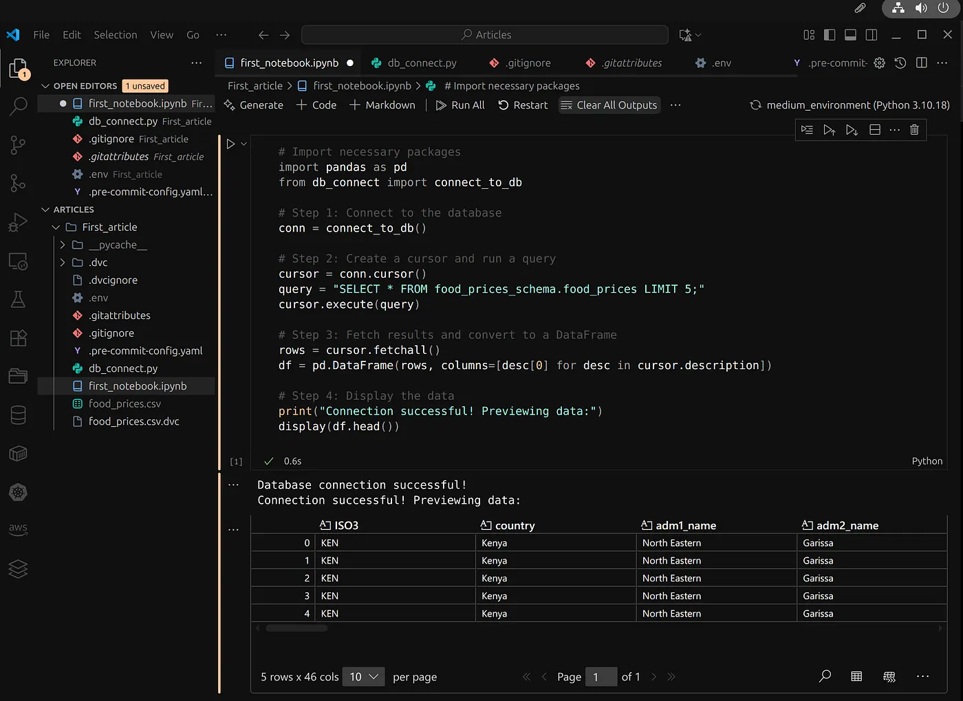
The data is seamlessly fetched from PostgreSQL and formatted directly inside your notebook!
The Output:
Locking Down Reproducibility
To ensure your environment can be reproduced by anyone on any machine, lock down your active Python libraries and version states into a single configuration file:
pip freeze > requirements.txt
When a collaborator clones your repository, they can instantly recreate your exact runtime workspace by running a single command: pip install -r requirements.txt.
Final Project Architecture
With our systems linked and our directory pipelines organized, your finished enterprise data workspace structure looks like this:
First_article/
├── data/
│   ├── 01-raw/                # Raw datasets (DVC managed, Git ignored)
│   ├── 02-preprocessed/       # Intermediate execution data
│   ├── 03-features/           # Modeled feature sets
│   └── 04-predictions/        # Pipeline outputs
├── notebooks/
│   └── EDA.ipynb              # Production-ready, auto-cleaned notebook
├── .dvc/                      # Data Version Control system configs
├── db_connect.py              # Central database utility engine
├── data.dvc                  # Lightweight tracking pointer file for data/
├── .env                       # Local secrets configuration (Git ignored)
├── .gitattributes             # Automation filters and cleaning hooks
├── .gitignore                 # File exclusions manifest
├── .pre-commit-config.yaml    # Automated pre-commit quality rules
└── requirements.txt           # Python dependency declarations
What Each File Does
| File / Folder | Purpose | |
|---|
| db_connect.py | Python script that manages database connections. | |
| first_notebook.ipynb | Main analysis or exploration notebook. | |
| food_prices.csv | Your dataset, versioned and tracked by DVC. | |
| food_prices.csv.dvc | Metadata file created by DVC to track dataset changes. | |
| .env | Contains environment variables (like database credentials). | |
| .dvc/ | Stores DVC’s internal configuration and cache tracking. | |
| .gitignore | Specifies files and folders Git should not track (like .env or caches). | |
| .gitattributes | Defines filters for Git LFS and nbstripout cleaning rules. | |
| .pre-commit-config.yaml | Holds pre-commit hook configurations to enforce clean commits. | |
| requirements.txt | Lists dependencies for reproducibility. | |
| pycache | Auto-generated by Python safe to ignore. | |
Conclusion & Next Steps
At this point, your data engineering environment matches the highest standards used across modern production data science teams. You have effectively:
-
Built a clean, compartmentalized multi-tier data directory pipeline.
-
Decoupled heavy storage tracking from Git using DVC.
-
Instituted a continuous validation pre-commit pipeline using nbstripout and nbQA.
-
Protected database configurations using secure local environment abstractions.
-
Connected Python cleanly to an active PostgreSQL service.
What’s Next?
-
Start executing exploratory data analysis (EDA) natively from your relational tables.
-
Build data processing scripts to clean your raw rows and output the results directly into your data/02-preprocessed/ directory.
-
Hook up analytical dashboards or serialization scripts to build data stories!