34 min read
Nairobi Airbnb Market Analysis
An end-to-end analysis of rental trends and pricing factors in Nairobi.
An end-to-end analysis of rental trends and pricing factors in Nairobi.
import numpy as np
import pandas as pd
import missingno as msno
import statsmodels.formula.api as smf
import matplotlib.pyplot as plt
import statsmodels.graphics.correlation as sgc
from statsmodels.graphics.gofplots import qqplot
import statsmodels.stats.api as sms
from statsmodels.stats.outliers_influence import OLSInfluence
from sklearn.preprocessing import StandardScaler
import seaborn as sns
from sklearn.model_selection import train_test_split
from sklearn.metrics import r2_score, mean_squared_error
from sklearn.tree import DecisionTreeRegressor
from sklearn.ensemble import RandomForestRegressorThis is the connection link to my database on postgreSQL, the actual connection function is on the file db_connect.py
# Import necessary packages
import pandas as pd
import sys
sys.path.append('..')  # Go up one level to the root folder
from db_connect import connect_to_db

# Step 1: Connect to the database
conn = connect_to_db()

# Step 2: Create a cursor and run a query
cursor = conn.cursor()
query = "SELECT * FROM airbnbs_nairobi.listing_data_yearly;"
cursor.execute(query)

# Step 3: Fetch results and convert to a DataFrame
rows = cursor.fetchall()
df = pd.DataFrame(rows, columns=[desc[0] for desc in cursor.description])

# Step 4: Display the data
print("Connection successful! Previewing data:")
display(df.head())
Database connection successful!
Connection successful! Previewing data:| listing_id | listing_name | listing_type | room_type | cover_photo_url | photos_count | minimum_nights | cancellation_policy | professional_management | registration | ... | rating_communication | rating_location | rating_value | revenue_per_year | avg_rate_per_year | annual_occupancy(%) | revenue_per_night_yearly | reserved_days_in_year | blocked_days_in_year | available_days_in_year | |
|---|---|---|---|---|---|---|---|---|---|---|---|---|---|---|---|---|---|---|---|---|---|
| 0 | 75683 | Kiloranhouse Apt Prime Bedroom | Private room in home | private_room | https://a0.muscache.com/im/pictures/5499026/ef... | 13 | 2 | Moderate | False | False | ... | 5.0 | 4.8 | 4.7 | 141049.0 | 6474.0 | 6.6 | 386.4 | 24 | 0 | 341 |
| 1 | 471581 | Located In a Serene Environment | Entire cottage | entire_home | https://a0.muscache.com/im/pictures/6434524/bc... | 37 | 2 | Moderate | False | False | ... | 4.9 | 4.8 | 4.8 | 804490.0 | 5791.6 | 54.8 | 3058.9 | 144 | 102 | 221 |
| 2 | 906958 | Makena's Place Karen - Flamingo Room | Private room in cottage | private_room | https://a0.muscache.com/im/pictures/68ecc57f-d... | 29 | 1 | Firm | False | False | ... | 4.9 | 4.9 | 4.9 | 594869.0 | 6772.2 | 24.4 | 1629.8 | 89 | 0 | 276 |
| 3 | 1023556 | Guesthouse Near Nairobi National Park & Airport | Entire guesthouse | entire_home | https://a0.muscache.com/im/pictures/ddd8badc-1... | 20 | 1 | Flexible | False | False | ... | 4.9 | 4.7 | 4.8 | 29004.0 | 3631.3 | 3.0 | 79.5 | 11 | 0 | 354 |
| 4 | 1237886 | Hob House | Room in bed and breakfast | hotel_room | https://a0.muscache.com/im/pictures/cbdab7e1-f... | 8 | 1 | Flexible | True | False | ... | 4.6 | 4.7 | 4.8 | 168583.0 | 15401.5 | 3.0 | 461.9 | 11 | 0 | 354 |
5 rows × 42 columns
df| listing_id | listing_name | listing_type | room_type | cover_photo_url | photos_count | minimum_nights | cancellation_policy | professional_management | registration | ... | rating_communication | rating_location | rating_value | revenue_per_year | avg_rate_per_year | annual_occupancy(%) | revenue_per_night_yearly | reserved_days_in_year | blocked_days_in_year | available_days_in_year | |
|---|---|---|---|---|---|---|---|---|---|---|---|---|---|---|---|---|---|---|---|---|---|
| 0 | 75683 | Kiloranhouse Apt Prime Bedroom | Private room in home | private_room | https://a0.muscache.com/im/pictures/5499026/ef... | 13 | 2 | Moderate | False | False | ... | 5.0 | 4.8 | 4.7 | 141049.0 | 6474.0 | 6.6 | 386.4 | 24 | 0 | 341 |
| 1 | 471581 | Located In a Serene Environment | Entire cottage | entire_home | https://a0.muscache.com/im/pictures/6434524/bc... | 37 | 2 | Moderate | False | False | ... | 4.9 | 4.8 | 4.8 | 804490.0 | 5791.6 | 54.8 | 3058.9 | 144 | 102 | 221 |
| 2 | 906958 | Makena's Place Karen - Flamingo Room | Private room in cottage | private_room | https://a0.muscache.com/im/pictures/68ecc57f-d... | 29 | 1 | Firm | False | False | ... | 4.9 | 4.9 | 4.9 | 594869.0 | 6772.2 | 24.4 | 1629.8 | 89 | 0 | 276 |
| 3 | 1023556 | Guesthouse Near Nairobi National Park & Airport | Entire guesthouse | entire_home | https://a0.muscache.com/im/pictures/ddd8badc-1... | 20 | 1 | Flexible | False | False | ... | 4.9 | 4.7 | 4.8 | 29004.0 | 3631.3 | 3.0 | 79.5 | 11 | 0 | 354 |
| 4 | 1237886 | Hob House | Room in bed and breakfast | hotel_room | https://a0.muscache.com/im/pictures/cbdab7e1-f... | 8 | 1 | Flexible | True | False | ... | 4.6 | 4.7 | 4.8 | 168583.0 | 15401.5 | 3.0 | 461.9 | 11 | 0 | 354 |
| ... | ... | ... | ... | ... | ... | ... | ... | ... | ... | ... | ... | ... | ... | ... | ... | ... | ... | ... | ... | ... | ... |
| 295 | 42123446 | Mvuli Luxury Suites | Entire rental unit | entire_home | https://a0.muscache.com/im/pictures/238557fd-c... | 24 | 1 | Firm | False | False | ... | 4.5 | 4.3 | 4.4 | 59105.0 | 3710.9 | 4.4 | 161.9 | 16 | 0 | 349 |
| 296 | 42139551 | Modern 1BR | King Bed | Fast Wi-Fi | Near CBD | Entire condo | entire_home | https://a0.muscache.com/im/pictures/a10f889a-4... | 27 | 1 | Flexible | False | False | ... | 4.9 | 4.9 | 4.8 | 228931.0 | 6572.8 | 9.0 | 663.6 | 31 | 20 | 334 |
| 297 | 42187559 | Cosy & Airy Studio with Balcony WI-FI and Netflix | Tiny home | entire_home | https://a0.muscache.com/im/pictures/miso/Hosti... | 43 | 1 | Moderate | True | False | ... | 5.0 | 4.7 | 5.0 | 25317.0 | 2041.4 | 3.3 | 69.4 | 12 | 0 | 353 |
| 298 | 42207619 | Kazuri Ivy Serene & Spacious Nairobi Apartment | Entire rental unit | entire_home | https://a0.muscache.com/im/pictures/hosting/Ho... | 19 | 2 | Moderate | False | False | ... | 4.9 | 4.4 | 4.8 | 422289.0 | 4969.1 | 25.6 | 1272.0 | 85 | 33 | 280 |
| 299 | 42223689 | Airy & Light-Filled: Indoor-Outdoor Home-Stay | Private room in rental unit | private_room | https://a0.muscache.com/im/pictures/fd146f8e-5... | 17 | 2 | Moderate | False | False | ... | 4.8 | 4.9 | 4.9 | 190766.0 | 2930.6 | 22.4 | 657.8 | 65 | 75 | 300 |
300 rows × 42 columns
df.info()<class 'pandas.core.frame.DataFrame'>
RangeIndex: 300 entries, 0 to 299
Data columns (total 42 columns):
# Column Non-Null Count Dtype
--- ------ -------------- -----
0 listing_id 300 non-null int64
1 listing_name 300 non-null object
2 listing_type 300 non-null object
3 room_type 300 non-null object
4 cover_photo_url 300 non-null object
5 photos_count 300 non-null int64
6 minimum_nights 300 non-null int64
7 cancellation_policy 300 non-null object
8 professional_management 300 non-null bool
9 registration 300 non-null bool
10 instant_book 300 non-null bool
11 amenities 300 non-null object
12 host_id 300 non-null int64
13 host_name 300 non-null object
14 cohost_ids 300 non-null object
15 cohost_names 300 non-null object
16 owned_by 300 non-null object
17 owners 300 non-null int64
18 superhost 300 non-null bool
19 latitude 300 non-null float64
20 longitude 300 non-null float64
21 guests_allowed 300 non-null int64
22 bedrooms 300 non-null int64
23 beds 300 non-null int64
24 baths 300 non-null float64
25 cleaning_fee 300 non-null float64
26 extra_guest_fee 300 non-null float64
27 num_reviews 300 non-null int64
28 rating_overall 300 non-null float64
29 rating_accuracy 300 non-null float64
30 rating_checkin 300 non-null float64
31 rating_cleanliness 300 non-null float64
32 rating_communication 300 non-null float64
33 rating_location 300 non-null float64
34 rating_value 300 non-null float64
35 revenue_per_year 300 non-null float64
36 avg_rate_per_year 300 non-null float64
37 annual_occupancy(%) 300 non-null float64
38 revenue_per_night_yearly 300 non-null float64
39 reserved_days_in_year 300 non-null int64
40 blocked_days_in_year 300 non-null int64
41 available_days_in_year 300 non-null int64
dtypes: bool(4), float64(16), int64(12), object(10)
memory usage: 90.4+ KBdf.describe()| listing_id | photos_count | minimum_nights | host_id | owners | latitude | longitude | guests_allowed | bedrooms | beds | ... | rating_communication | rating_location | rating_value | revenue_per_year | avg_rate_per_year | annual_occupancy(%) | revenue_per_night_yearly | reserved_days_in_year | blocked_days_in_year | available_days_in_year | |
|---|---|---|---|---|---|---|---|---|---|---|---|---|---|---|---|---|---|---|---|---|---|
| count | 3.000000e+02 | 300.000000 | 300.000000 | 3.000000e+02 | 300.000000 | 300.000000 | 300.000000 | 300.000000 | 300.000000 | 300.000000 | ... | 300.000000 | 300.000000 | 300.000000 | 3.000000e+02 | 300.000000 | 300.000000 | 300.000000 | 300.000000 | 300.000000 | 300.000000 |
| mean | 2.818099e+07 | 30.100000 | 2.176667 | 1.294209e+08 | 1.580000 | -1.282688 | 36.793314 | 5.360000 | 1.736667 | 2.176667 | ... | 4.869000 | 4.825333 | 4.775000 | 5.557893e+05 | 7504.654667 | 23.385333 | 1733.102333 | 73.513333 | 39.670000 | 291.486667 |
| std | 1.191095e+07 | 16.297916 | 3.445533 | 1.062699e+08 | 0.890455 | 0.035017 | 0.039478 | 4.856854 | 1.571269 | 2.031225 | ... | 0.157549 | 0.174527 | 0.194769 | 8.759067e+05 | 6837.522117 | 20.727560 | 2581.110728 | 66.100738 | 52.670057 | 66.100738 |
| min | 7.568300e+04 | 0.000000 | 1.000000 | 2.699700e+04 | 1.000000 | -1.379600 | 36.669400 | 1.000000 | 0.000000 | 1.000000 | ... | 3.700000 | 3.600000 | 3.000000 | 1.826400e+04 | 1366.000000 | 2.700000 | 50.000000 | 10.000000 | 0.000000 | 34.000000 |
| 25% | 2.000117e+07 | 19.000000 | 1.000000 | 3.594571e+07 | 1.000000 | -1.297350 | 36.779075 | 2.000000 | 1.000000 | 1.000000 | ... | 4.800000 | 4.800000 | 4.700000 | 1.338565e+05 | 4382.800000 | 6.675000 | 399.450000 | 22.000000 | 0.000000 | 261.000000 |
| 50% | 3.198200e+07 | 28.000000 | 1.000000 | 1.008633e+08 | 1.000000 | -1.284950 | 36.791200 | 4.000000 | 1.000000 | 2.000000 | ... | 4.900000 | 4.900000 | 4.800000 | 3.001395e+05 | 6198.150000 | 15.700000 | 950.500000 | 50.000000 | 20.000000 | 315.000000 |
| 75% | 3.868569e+07 | 37.000000 | 2.000000 | 2.237596e+08 | 2.000000 | -1.264500 | 36.806925 | 6.000000 | 2.000000 | 3.000000 | ... | 5.000000 | 4.900000 | 4.900000 | 6.591980e+05 | 8770.775000 | 35.100000 | 2171.350000 | 104.000000 | 61.250000 | 343.000000 |
| max | 4.222369e+07 | 122.000000 | 30.000000 | 4.292661e+08 | 6.000000 | -1.187200 | 36.909600 | 16.000000 | 15.000000 | 19.000000 | ... | 5.000000 | 5.000000 | 5.000000 | 1.070000e+07 | 88421.700000 | 90.700000 | 32344.600000 | 331.000000 | 258.000000 | 355.000000 |
8 rows × 28 columns
import re

def to_snake_case(name):
    # Convert to lowercase
    name = name.lower()
    # Replace spaces with underscores
    name = name.replace(' ', '_')
    # Remove special characters like parentheses
    name = re.sub(r'[(%\)]+', '', name)
    # Replace multiple underscores with single underscore
    name = re.sub(r'_+', '_', name)
    return name

# Apply to all columns
df.columns = [to_snake_case(col) for col in df.columns]

print(df.columns)
Index(['listing_id', 'listing_name', 'listing_type', 'room_type',
'cover_photo_url', 'photos_count', 'minimum_nights',
'cancellation_policy', 'professional_management', 'registration',
'instant_book', 'amenities', 'host_id', 'host_name', 'cohost_ids',
'cohost_names', 'owned_by', 'owners', 'superhost', 'latitude',
'longitude', 'guests_allowed', 'bedrooms', 'beds', 'baths',
'cleaning_fee_', 'extra_guest_fee', 'num_reviews', 'rating_overall',
'rating_accuracy', 'rating_checkin', 'rating_cleanliness',
'rating_communication', 'rating_location', 'rating_value',
'revenue_per_year', 'avg_rate_per_year', 'annual_occupancy',
'revenue_per_night_yearly', 'reserved_days_in_year',
'blocked_days_in_year', 'available_days_in_year'],
dtype='object')msno.matrix(df)<Axes: >
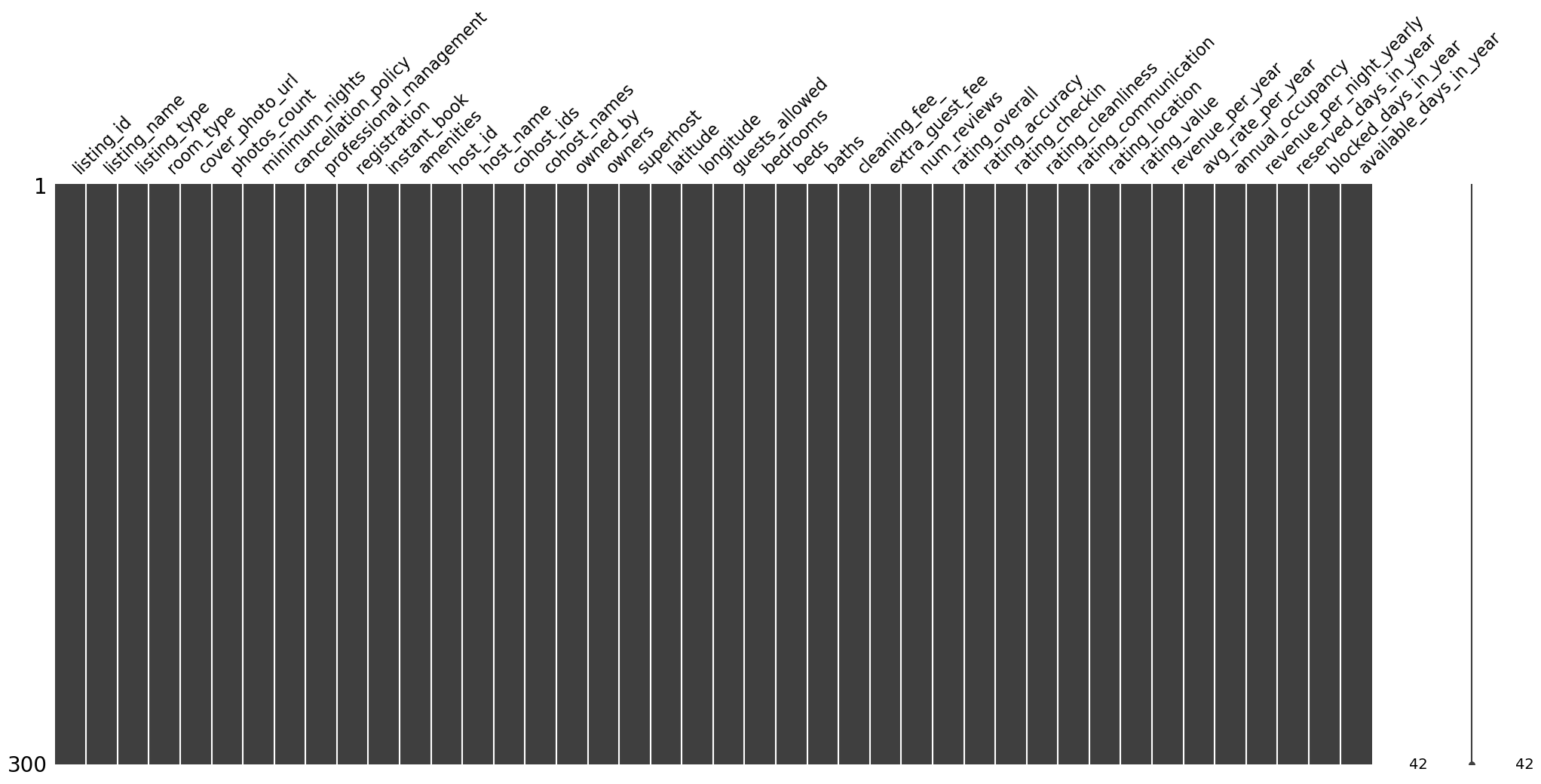 representation of all columns to show no missing value
For this analysis, room type is used as the primary classification variable, as it provides a more general and consistent categorization of listings. In contrast, listing type contains a large number of highly specific categories, which can introduce unnecessary complexity and reduce comparability across observations.
listing_type = df['listing_type'].unique()
len(listing_type)29room_type = df['room_type'].unique()
len(room_type)
room_typearray(['private_room', 'entire_home', 'hotel_room'], dtype=object)While listing types consist of 29 unique categories across the dataset, room types are limited to three broad and representative categories that better capture the nature of the accommodation. These include Private Room, Entire Home/Apartment, and Hotel Room, the latter of which appears only once in the dataset.
room_type_count = df['room_type'].value_counts()
plt.figure(figsize=(10,8))
plt.pie(room_type_count, labels=room_type_count.index, colors=("#0FB9B9", "#E29015", "#F3013E"), autopct='%1.1f%%', startangle=90, textprops={'fontsize':11})
plt.title("Room Type Distribution Across the Dataset", fontsize=12, fontweight='bold')
plt.tight_layout()
plt.show()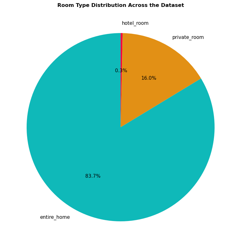 A pie chart visualizing the distribution of room types
listing_type_vs_avg_rate_per_night = df.groupby('room_type')['avg_rate_per_year'].mean().sort_values(ascending=False).round(2)
plt.figure(figsize=(10, 6))
listing_type_vs_avg_rate_per_night.plot(kind='bar', color=["#1AF64D", "#10EFCD", "#F60F0FF3"])
plt.title('Listing Type correlation to Average Rate Per Night', fontsize=14, fontweight='bold')
plt.ylabel('Average rate per Night', fontsize=14)
plt.xlabel('Type of Listing', fontsize=14)
plt.xticks(rotation=0)
plt.tight_layout()
plt.show()
# display the findings
listing_type_vs_avg_rate_per_night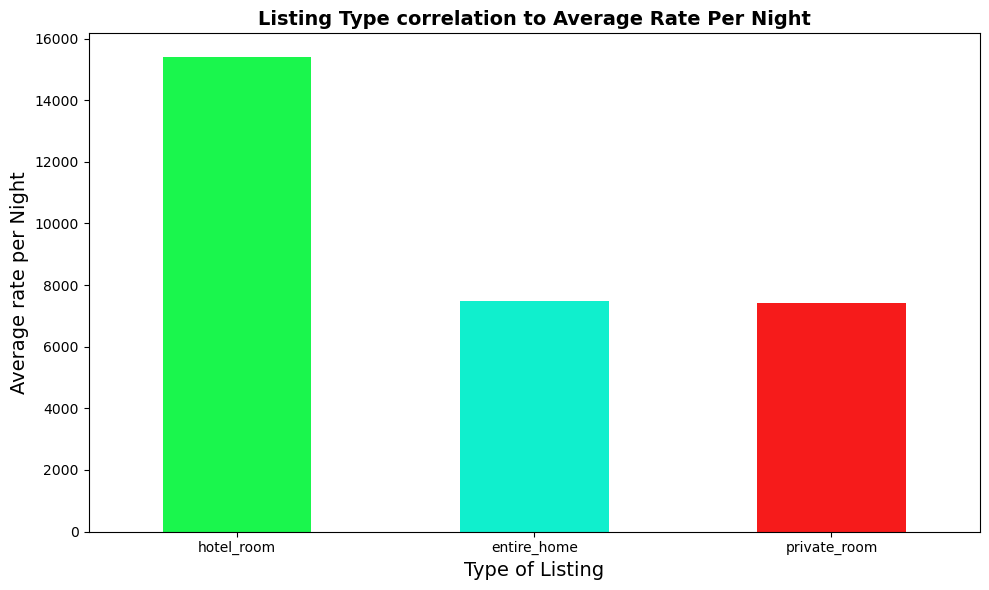 a bar chart visualizing listing type and their average rate per night
room_type
hotel_room      15401.50
entire_home      7488.58
private_room     7424.20
Name: avg_rate_per_year, dtype: float64
Based on the analysis, hotel rooms command the highest average nightly rate at KSh 15,401. In contrast, entire homes and private rooms are priced at relatively similar levels, with average nightly rates of KSh 7,488 and KSh 7,424, respectively.
avg_rate_vs_revenue_per_room_type = df.groupby('room_type')['revenue_per_year'].mean().sort_values(ascending=False).round(2)
avg_rate_vs_revenue_per_room_type
room_type
entire_home 619762.21
private_room 229331.23
hotel_room 168583.00
Name: revenue_per_year, dtype: float64avg_rate_vs_revenue_per_room_type = (
df.groupby('room_type')
.agg(
avg_rate_per_night=('avg_rate_per_year', 'mean'),
revenue_per_year=('revenue_per_year', 'mean')
)
).sort_values(by='revenue_per_year', ascending=False).round(2)
avg_rate_vs_revenue_per_room_type| avg_rate_per_night | revenue_per_year | |
|---|---|---|
| room_type | ||
| entire_home | 7488.58 | 619762.21 |
| private_room | 7424.20 | 229331.23 |
| hotel_room | 15401.50 | 168583.00 |
The listing type generating the most revenue is Entire Home, Ksh 619762 despite being the second highest rate per night, followed by Private Room generating Ksh 229331 per year and lastly Hotel Rooms generating Ksh 168583 despite being the highest rate per night
A listing is considered professionally managed when it is:
Operated by a property management company or hospitality firm
Managed by hosts who handle multiple properties as a business rather than a single personal residence
This typically includes:
Standardized check-in/check-out procedures
Dedicated cleaning and maintenance teams
Consistent pricing and availability management
Formal guest communication and support systems
How this differs from individual hosts
Individually managed listings are usually run by:
A single host
Often the property owner
With more personalized and less standardized operations
Professionally managed listings tend to:
Have stricter policies (e.g., cancellation, minimum nights)
Operate more like hotels or serviced apartments
Prioritize occupancy optimization and operational efficiency
# Map boolean values to labels
management_labels = df['professional_management'].map({
    True: 'Professionally Managed',
    False: 'Individually Managed'
})

professional_management_pie = management_labels.value_counts()

colors = ("#5da718", "#79059c")

plt.figure(figsize=(10, 8))
plt.pie(
    professional_management_pie,
    labels=professional_management_pie.index,
    autopct='%1.1f%%',
    colors=colors,
    startangle=90,
    textprops={'fontsize': 11}
)
plt.title("Professionally Managed vs Individually Managed Listings")
plt.tight_layout()
plt.show()

# Display counts
print(professional_management_pie)
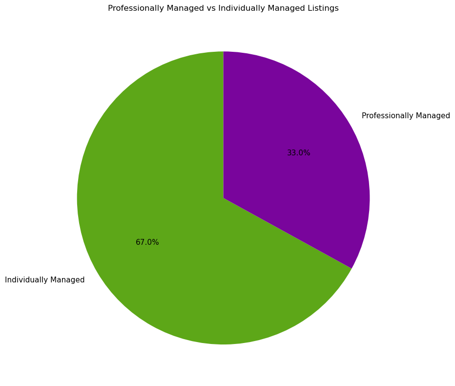 A pie chart visualising distribution of how listings are managed
professional_management
Individually Managed      201
Professionally Managed     99
Name: count, dtype: int64
so 99 Listings making up 33% of all the listings are professionally managed while 201 Listings making uo 67% of all the listings are Individually managed
management_labels = df['professional_management'].map({
True: 'Professionally Managed',
False: 'Individually Managed'
})
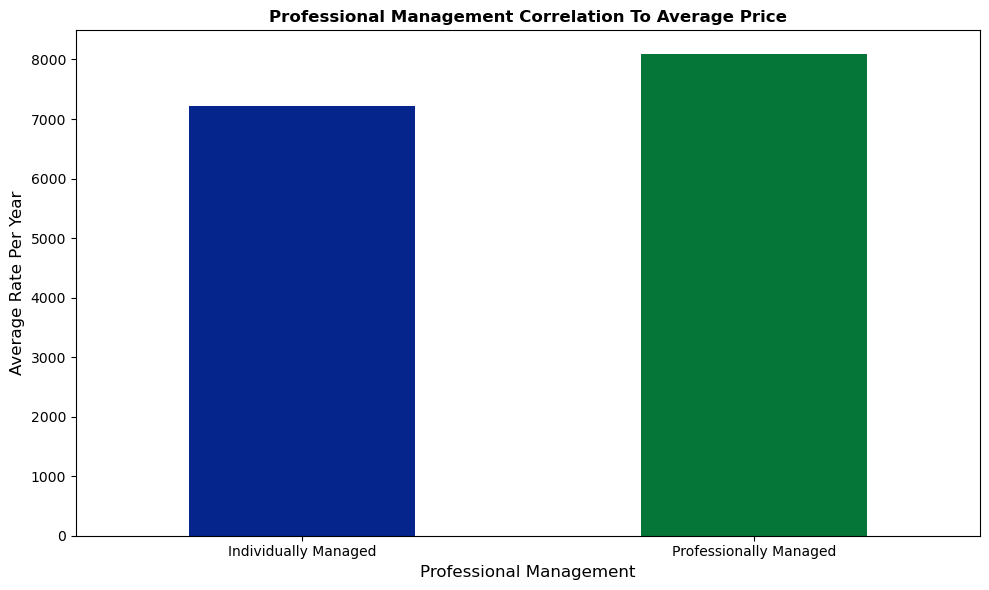
pricing_vs_avg_rate_per_year = df.groupby(management_labels)['avg_rate_per_year'].mean().round(2)
pricing_vs_avg_rate_per_yearprofessional_management
Individually Managed 7218.56
Professionally Managed 8085.51
Name: avg_rate_per_year, dtype: float64plt.figure(figsize=(10,6))
pricing_vs_avg_rate_per_year.plot(kind='bar', color=["#05258D","#067538"])
plt.title('Professional Management Correlation To Average Price', fontsize=12, fontweight='bold')
plt.xlabel('Professional Management', fontsize=12)
plt.xticks(rotation=0)
plt.ylabel('Average Rate Per Year', fontsize=12)
plt.tight_layout()
plt.show()
 A bar chart showing how differently managed listings rate
based on our chart above, the professionally managed listings tend to be priced higher compared to individually run listings, With professionally managed listings charging an average a rate of 8086 per Night and Individually Managed Listings charging an average rate of 7219 per Night
professionally_managed_vs_reviews = df.groupby(management_labels)['rating_overall'].mean().sort_values(ascending=True).round(2)
professionally_managed_vs_reviews
professional_management
Professionally Managed 4.77
Individually Managed 4.79
Name: rating_overall, dtype: float64Individually Managed Listings are slightly better rated at 4.79 compared to Professionally Managed listings at 4.77
To assess whether host management strategy influences booking flexibility, we examined the distribution of cancellation policies across professionally and individually managed listings.
professional_management_vs_cancellation_strictness = df.groupby('cancellation_policy')['professional_management'].value_counts
professional_management_vs_cancellation_strictness
<bound method SeriesGroupBy.value_counts of <pandas.core.groupby.generic.SeriesGroupBy object at 0x79cb866339e0>>pm_vs_policy = (
pd.crosstab(
df['cancellation_policy'],
df['professional_management'].map({
True: 'Professionally Managed',
False: 'Individually Managed'
})
)
)
pm_vs_policy.plot(
    kind='bar',
    stacked=True,
    figsize=(10, 6)
)

plt.title('Professional Management vs Cancellation Policy')
plt.xlabel('Cancellation Policy')
plt.ylabel('Number of Listings')
plt.xticks(rotation=0)
plt.tight_layout()
plt.show()
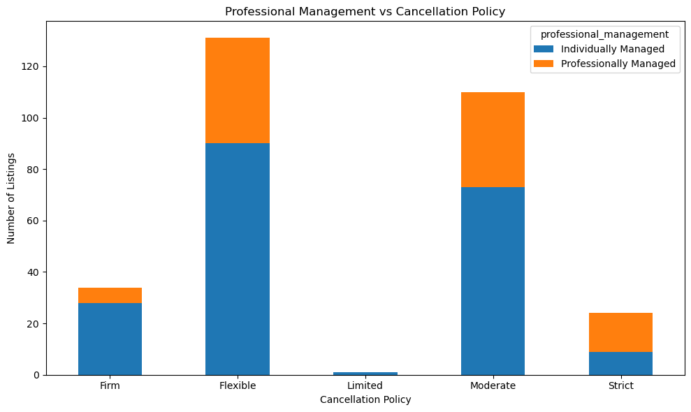 A stacked bar chart showing which cancellation policy listings fall under and their management category
Flexible policies are dominated by individually managed listingsThe majority of listings with Flexible cancellation policies are individually managed, suggesting that solo hosts prioritize flexibility to attract bookings and remain competitive.
Professionally managed listings are more concentrated in stricter policiesUnder Strict and Moderate cancellation policies, professionally managed listings make up a noticeably larger share. This indicates that professional operators are more comfortable enforcing stricter terms, likely due to better demand forecasting, operational buffers, and portfolio diversification.
Moderate policies represent a middle ground for both host typesBoth individual and professional hosts are strongly represented under Moderate policies, reinforcing the idea that this policy balances guest appeal with revenue protection.
Firm and Limited policies are relatively rareVery few listings adopt Firm or Limited cancellation policies, suggesting low market preference—possibly due to reduced guest willingness to book under highly restrictive conditions.
Overall, professional management is associated with stricter cancellation strategies, while individual hosts rely more on flexibility to drive demand. This highlights differing risk tolerance and pricing strategies between professional operators and independent hosts in Nairobi’s Airbnb market.
If you want, I can now help you connect this insight directly to pricing or occupancy outcomes for a stronger narrative in your report.
# Create price bins
df['price_range'] = pd.cut(df['avg_rate_per_year'],
                            bins=[0, 5000, 10000, 15000, 20000],
                            labels=['Budget (0-5k)', 'Mid-range (5-10k)', 'Premium (10-15k)', 'Luxury (15k+)'])

# Group by price range
best_price_metric = df.groupby('price_range')['annual_occupancy'].agg(['mean', 'count']).sort_values('mean', ascending=False)

plt.figure(figsize=(10, 6))
best_price_metric['mean'].plot(kind='bar', color='steelblue')
plt.title('Average Occupancy by Price Range', fontsize=16, fontweight='bold')
plt.xlabel('Price Range', fontsize=14)
plt.ylabel('Average Occupancy (%)', fontsize=14)
plt.xticks(rotation=0)
plt.tight_layout()
plt.show()

print(best_price_metric)
/tmp/ipykernel_54075/1302887327.py:7: FutureWarning: The default of observed=False is deprecated and will be changed to True in a future version of pandas. Pass observed=False to retain current behavior or observed=True to adopt the future default and silence this warning.
best_price_metric = df.groupby('price_range')['annual_occupancy'].agg(['mean', 'count']).sort_values('mean', ascending=False)
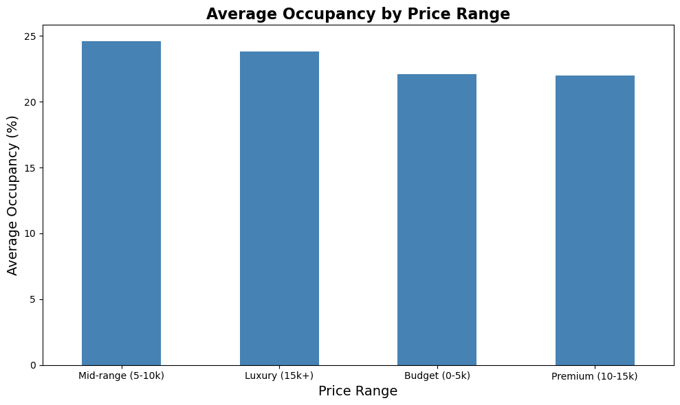 Different price bins and the occupancy rate they attract
                        mean  count
price_range
Mid-range (5-10k)  24.607586    145
Luxury (15k+)      23.842857     14
Budget (0-5k)      22.109615    104
Premium (10-15k) 22.013333 30Mid-range listings (KSh 5k–10k) attract the most customersWith the highest average occupancy, mid-range listings appear to offer the best balance between price and perceived value. This price segment is likely the most attractive to the majority of guests in Nairobi.
Luxury listings (KSh 15k+) maintain strong demandDespite higher prices, luxury listings show relatively high occupancy, suggesting a consistent market for premium accommodation—possibly driven by business travelers, expatriates, or high-end tourists.
Budget listings (Below KSh 5k) do not achieve the highest occupancyWhile budget listings are cheaper, their lower occupancy compared to mid-range listings suggests that price alone is not the primary driver of demand. Factors such as location, amenities, and perceived quality likely play a significant role.
Premium listings (KSh 10k–15k) show moderate occupancyPremium listings fall between mid-range and budget listings in terms of occupancy, indicating that demand tapers slightly as prices rise beyond the mid-range threshold.
Mid-range Airbnb listings (KSh 5k–10k) attract the highest customer demand, highlighting a value-for-money sweet spot in Nairobi’s short-term rental market.
In this segment, we check the various types of cancellation policies present within our dataset
plt.figure(figsize=(10, 8))
cancellation_policy_count = df['cancellation_policy'].value_counts()
colors = ['#FF6B6B', "#6F0DD0", '#45B7D1', "#EDC914", "#4EED14"]
plt.pie(cancellation_policy_count, labels=cancellation_policy_count.index, autopct='%1.1f%%',
colors=colors, startangle=90, textprops={'fontsize': 11})
plt.title("Cancellation Policy Distribution", fontsize=14, fontweight='bold')
plt.tight_layout()
plt.show()
# Display the counts
print(cancellation_policy_count)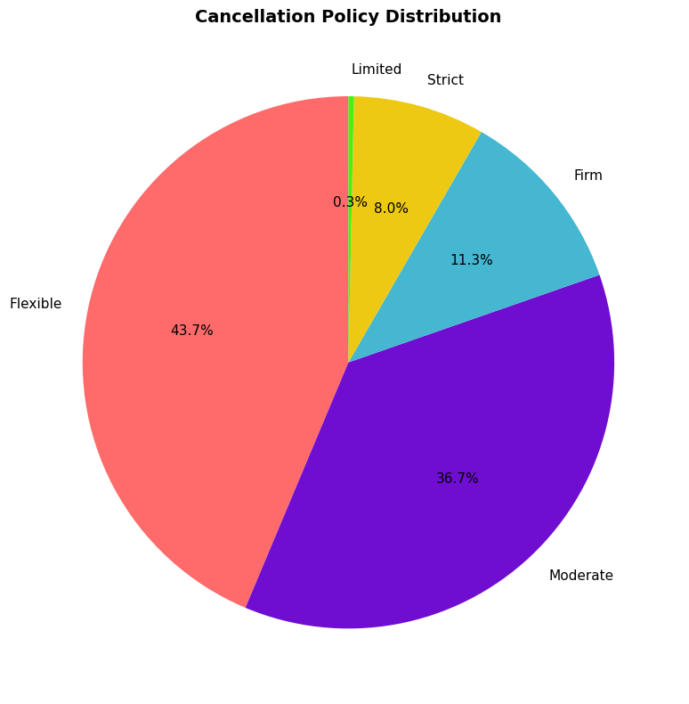 A distribution of different cancellation policies throughout our listings
cancellation_policy
Flexible    131
Moderate    110
Firm         34
Strict       24
Limited       1
Name: count, dtype: int64The dataset is dominated by Flexible and Moderate cancellation policies, with 43.7% and 36.7% listings respectively. This suggests that most hosts prefer policies that allow guests greater freedom to cancel reservations with minimal penalties.
Firm and Strict policies are less common, appearing in 11.3% and 8.0% listings respectively, indicating a smaller segment of hosts who prioritize booking certainty over flexibility.
Only one listing follows a Limited cancellation policy, making it negligible in the overall distribution.
Overall, the distribution reflects a guest-friendly marketplace, where flexible cancellation options are more prevalent than restrictive policies, likely aimed at attracting short-term and undecided travelers.
valid_policies = ['Flexible', 'Moderate', 'Firm', 'Strict']
cancellation_policy_vs_pricing = df[df['cancellation_policy'].isin(valid_policies)].groupby('cancellation_policy')['avg_rate_per_year'].mean().sort_values(ascending=False).round(2)
cancellation_policy_vs_pricing
cancellation_policy
Moderate 8850.24
Strict 7568.66
Firm 6986.59
Flexible 6418.48
Name: avg_rate_per_year, dtype: float64so i got rid of Limited since it’s only one entry, i don’t think it a good representation of the insights i’d like to derive from the dataset
plt.figure(figsize=(10,6))
cancellation_policy_vs_pricing.plot(kind='bar')
plt.title('Cancellation Policy and it\'s effect on Pricing of the Listing',fontsize=14,fontweight='bold' )
plt.ylabel('Average Rate per Night', fontsize=12)
plt.xlabel('Cancellation Policy', fontsize=12)
plt.xticks(rotation=0)
plt.tight_layout()
plt.show()
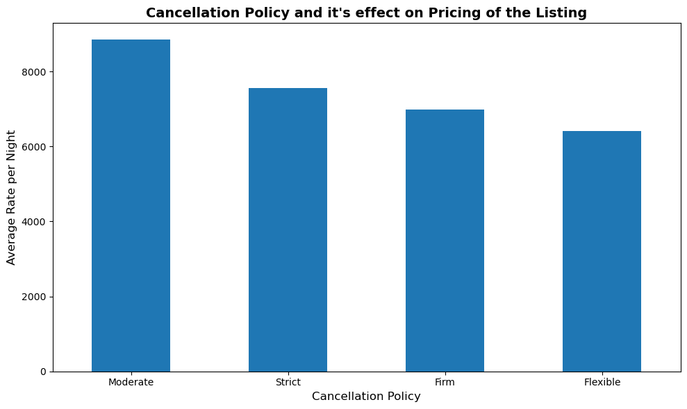 Different cancellation policies and the price rate they attract
The chart shows a clear relationship between cancellation strictness and average nightly price.
Moderate cancellation policies have the highest average nightly rates, suggesting that hosts with mid-level flexibility are able to charge a premium—possibly balancing guest trust with revenue protection.
Strict policies follow closely, indicating that listings enforcing tighter cancellation rules still command relatively high prices, likely due to stronger demand, desirable locations, or higher-quality listings.
Firm policies sit in the middle range, reflecting a moderate pricing strategy.
Flexible cancellation policies are associated with the lowest average nightly rates, suggesting that hosts may lower prices to compensate for the higher risk of last-minute cancellations.
Overall, less flexible cancellation policies tend to correlate with higher pricing, implying that hosts who restrict cancellations may do so confidently when their listings have strong market appeal. Conversely, greater flexibility appears to be used as a competitive pricing lever to attract more bookings.
The average occupancy rate across all active Airbnb listings in Nairobi provides a baseline measure of market demand. This metric helps contextualize how different pricing strategies, room types, and cancellation policies perform relative to the overall market.
average_occupancy_rate = df['annual_occupancy'].mean().round(2)
average_occupancy_ratenp.float64(23.39)Average occupancy rate across the dataset is 23.39%
valid_policies = ['Flexible', 'Moderate', 'Firm', 'Strict']
cancellation_policy_vs_occupancy = df[df['cancellation_policy'].isin(valid_policies)].groupby('cancellation_policy')['annual_occupancy'].mean().sort_values(ascending=False).round(2)
cancellation_policy_vs_occupancy
cancellation_policy
Strict 26.35
Moderate 23.61
Firm 23.29
Flexible 22.42
Name: annual_occupancy, dtype: float64From our Findings,Listings with Strict cancellation policy holds the largest percentage of annual occupancy rate at 26.35%, Listings with Moderate cancellation policy come in second with 23.61%, Firm Cancellation policy listings hold a 23.29% annual occupancy rate and listings with Flexible cancellation Policy hold the least annual occupancy percentage at 22.42%. So to answer the question, No
minimum_nights_vs_booking_frequency = df.groupby('minimum_nights')['annual_occupancy'].mean().sort_values(ascending=False)
minimum_nights_vs_booking_frequency
minimum_nights
30 81.600000
28 43.850000
7 30.800000
3 29.932258
2 26.201031
1 19.886275
4 13.850000
14 4.200000
5 3.600000
Name: annual_occupancy, dtype: float64plt.figure(figsize=(10,6))
minimum_nights_vs_booking_frequency.plot(kind='barh')
plt.title('Minimum Nights vs Booking Frequency', fontsize=14, fontweight='bold')
plt.ylabel('Minimum Nights', fontsize=12)
plt.xlabel('Annual Occupancy Percentage', fontsize=12)
plt.tight_layout()
plt.show()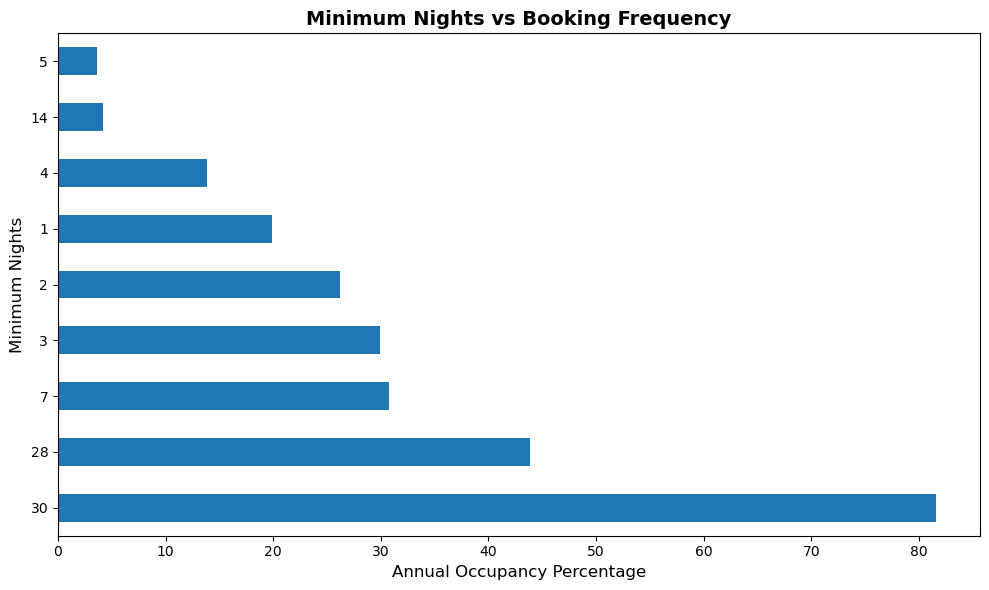 A horizontal bar showing minimum nights requirement and the occupancy rate they attract
1. Long-Term Stays Dominate Annual Occupancy
30-Day Stays are King: The most significant finding is that bookings with a minimum stay of 30 nights account for the highest annual occupancy percentage by a wide margin, reaching approximately 82%.
Strong Performance of 28-Day Stays: The second-highest occupancy is for 28-night minimum stays, at around 44%.
Conclusion: This suggests a very strong market for monthly or near-monthly rentals, which could be driven by corporate housing, digital nomads, or temporary relocations. These long stays are the primary drivers of occupancy in this dataset.
2. Weekly and Long-Weekend Stays are Important Secondary Drivers
The “Sweet Spot” for Shorter Stays: Minimum stays of 7 nights and 3 nights have very similar and significant occupancy percentages, both hovering around the 30-31% mark.
Conclusion: There is substantial demand for weekly vacations and extended weekend trips. For hosts not targeting the monthly market, these two durations appear to be the most effective for maintaining occupancy.
3. Very Short Stays Contribute Less to Overall Occupancy
1-2 Night Stays: While extremely common in the short-term rental market, minimum stays of 2 nights (~26%) and 1 night (~20%) contribute less to the total annual occupancy than the 3, 7, 28, and 30-night options.
Implication: This could indicate that while these bookings may be frequent, the higher turnover results in more unbooked “gap days,” leading to a lower overall occupancy percentage over the course of a year compared to longer, more continuous stays.
4. Specific Durations are Less Effective
Low Occupancy for 4, 5, and 14 Nights: Minimum stays of 4 nights (~14%), 14 nights (~4%), and 5 nights (~3%) show the lowest annual occupancy percentages.
Conclusion: These specific booking windows seem to be less popular with guests or less successfully utilized by hosts compared to the standard 1-night, weekend (2-3 nights), weekly (7 nights), or monthly models.
Strategic Implication for Hosts: To maximize annual occupancy, the data suggests targeting the 30+ day market is the most effective strategy. If that is not feasible, focusing on 7-night (weekly) or 3-night (long weekend) minimums would be better than setting minimums of 1, 2, 4, 5, or 14 nights.
Key Insight The data suggests that decreasing booking frequency (by raising minimum nights to 28+) actually increases your overall business performance (occupancy).
listing_types_vs_occupancy_rate = df.groupby('room_type')['annual_occupancy'].mean().sort_values(ascending=False).round(2)
listing_types_vs_occupancy_rate
room_type
entire_home 25.05
private_room 15.08
hotel_room 3.00
Name: annual_occupancy, dtype: float64Entire Homes are the most common listing type to be booked at a rate of 25.05%, followed by Private Room at a rate of 15.08% and lastlyHotel Rooms making up 3.0% of the total occupancy rate
no_of_hosts = df['host_id'].unique()
len(no_of_hosts)205Our dataset has 205 unique hosts all who own either one or a bunch of listings within Nairobi
no_of_listing_per_host = (
    df.groupby('host_id')
      .agg(
          host_name=('host_name', 'first'),
          number_of_listings=('listing_id', 'count')
      ).sort_values(by='number_of_listings',ascending=False)
)

no_of_listing_per_host| host_name | number_of_listings | |
|---|---|---|
| host_id | ||
| 35945714 | Samra Apartments | 19 |
| 308523342 | Damaris | 8 |
| 8042369 | Sherry | 7 |
| 145631743 | Diana | 6 |
| 43851715 | Duncan | 5 |
| ... | ... | ... |
| 322215915 | David | 1 |
| 326653326 | Alain | 1 |
| 327031637 | Lillian | 1 |
| 363302880 | Nyangaga | 1 |
| 429266147 | Anata | 1 |
205 rows × 2 columns
top_host = no_of_listing_per_host.iloc[0]
print(f"Top host: {top_host['host_name']} with {top_host['number_of_listings']} listings")
Top host: Samra Apartments with 19 listingsprint(f"Total hosts: {len(no_of_listing_per_host)}")
print(f"Average listings per host: {no_of_listing_per_host['number_of_listings'].mean():.2f}")
print(f"Max listings by one host: {no_of_listing_per_host['number_of_listings'].max()}")
print(f"Min listings by one host: {no_of_listing_per_host['number_of_listings'].min()}")Total hosts: 205
Average listings per host: 1.46
Max listings by one host: 19
Min listings by one host: 1The dataset contains 205 unique hosts, with an average of 1.46 listings per host, indicating that the market is largely composed of small-scale hosts. Most hosts operate a single listing, as reflected by the minimum of one listing per host. However, there is evidence of professional or portfolio-style hosting, with the largest host, Samra Apartments, managing 19 listings. This highlights a market structure dominated by individual hosts alongside a small number of high-volume operators.
plt.figure(figsize=(8, 6))
plt.scatter(df['longitude'], df['latitude'], c=df['avg_rate_per_year'], alpha=0.6)
plt.colorbar(label='Average Nightly Rate')
plt.xlabel('Longitude')
plt.ylabel('Latitude')
plt.title('Pricing Distribution Across Nairobi')
plt.show()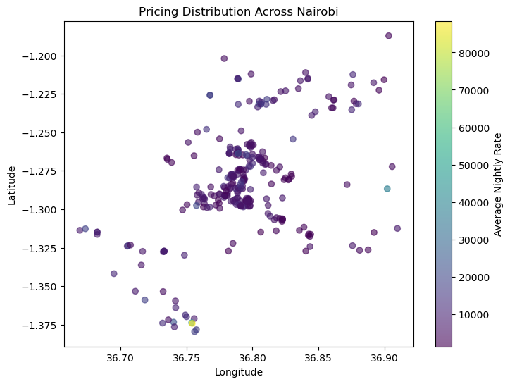 A distribution of our listings
NAIROBI_BOUNDS = {
    "lat_min": -1.5,
    "lat_max": -1.1,
    "lon_min": 36.6,
    "lon_max": 37.1
}
df_nairobi = df[
    (df['latitude'] >= NAIROBI_BOUNDS['lat_min']) &
    (df['latitude'] <= NAIROBI_BOUNDS['lat_max']) &
    (df['longitude'] >= NAIROBI_BOUNDS['lon_min']) &
    (df['longitude'] <= NAIROBI_BOUNDS['lon_max'])
].copy()

print(f"Listings before: {len(df)}")
print(f"Listings in Nairobi: {len(df_nairobi)}")
Listings before: 300
Listings in Nairobi: 300
import folium
from IPython.display import display
m = folium.Map(
location=[-1.286389, 36.817223], # Nairobi CBD
zoom_start=12,
min_zoom=11,
max_zoom=16,
max_bounds=True,
bounds=NAIROBI_BOUNDS,
tiles="OpenStreetMap"
)
#m.fit_bounds(NAIROBI_BOUNDS)for row in df_nairobi.itertuples():
if row.avg_rate_per_year < 5000:
color = '#2EC4B6' # Budget
elif row.avg_rate_per_year < 10000:
color = '#1F77B4' # Mid-range
elif row.avg_rate_per_year < 15000:
color = '#FF9F1C' # Premium
else:
color = '#E63946' # Luxury
# Create popup with more details
popup_text = f"""
<b style='font-size: 14px'>{row.listing_name}</b><br>
<b>Type:</b> {row.listing_type}<br>
<b>Room:</b> {row.room_type}<br>
<b>Rating:</b> {row.rating_overall}/5.0<br>
<b>Price:</b> KSh {row.avg_rate_per_year:.0f}/night
"""
folium.CircleMarker(
location=[row.latitude, row.longitude],
radius=4,
color=color,
fill=True,
fill_color=color,
fill_opacity=0.7,
popup=folium.Popup(popup_text, max_width=300)
).add_to(m)
display(m)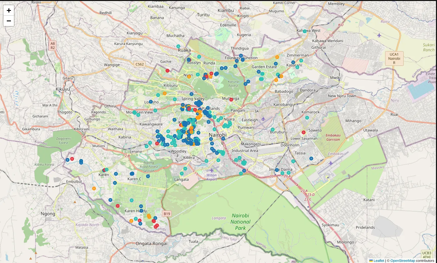
from sklearn.cluster import KMeans
from sklearn.preprocessing import StandardScaler

X = neighbourhoods_vs_pricing[['avg_rate_per_year']]

scaler = StandardScaler()
X_scaled = scaler.fit_transform(X)kmeans = KMeans(n_clusters=3, random_state=42)
neighbourhoods_vs_pricing['price_cluster'] = kmeans.fit_predict(X_scaled)
neighbourhoods_vs_pricing.sort_values('avg_rate_per_year')| suburb | avg_rate_per_year | price_cluster | |
|---|---|---|---|
| 0 | Nyayo Highrise ward | 1427.50 | 0 |
| 1 | South C | 1717.10 | 0 |
| 2 | Pipeline | 1819.50 | 0 |
| 3 | South B | 2341.67 | 0 |
| 4 | Mugumo-ini ward | 2796.90 | 0 |
| 5 | Nairobi West | 2857.30 | 0 |
| 6 | CBD division | 3373.79 | 0 |
| 7 | Komarock ward | 4296.90 | 0 |
| 8 | Imara Daima ward | 4452.97 | 0 |
| 9 | Harambee ward | 4460.60 | 0 |
| 10 | Githurai division | 5098.80 | 0 |
| 11 | South C ward | 5177.70 | 0 |
| 12 | Kangemi division | 5242.46 | 0 |
| 13 | Nairobi West ward | 5552.50 | 0 |
| 14 | Kawangware division | 5684.97 | 0 |
| 15 | Roysambu division | 6030.61 | 0 |
| 16 | Woodley/Kenyatta/Golf Course ward | 6614.90 | 2 |
| 17 | Kasarani location | 6667.00 | 2 |
| 18 | Kilimani division | 7002.30 | 2 |
| 19 | Tassia | 7173.10 | 2 |
| 20 | Highridge division | 8471.39 | 2 |
| 21 | Karen C | 8600.96 | 2 |
| 22 | Karen | 8606.50 | 2 |
| 23 | Karen Hardy | 10907.72 | 2 |
| 24 | Karen ward | 17108.63 | 2 |
| 25 | Lower Savannah ward | 37484.90 | 1 |
sns.barplot(
    data=neighbourhoods_vs_pricing,
    x='price_cluster',
    y='avg_rate_per_year'
)
plt.title("Average Nightly Rate by Neighborhood Price Cluster")
plt.show()
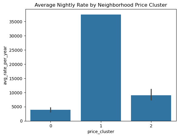 Price clusters and the rate they fall under
Cluster 0 (Economy/Budget): This category contains the highest volume of listings, representing the lower-tier accommodations.
Cluster 2 (Mid-range): These listings represent the middle tier of the market.
Cluster 1 (High-end/Outlier): This cluster contains only a single listing, suggesting it is unique or an outlier.”
neighborhood_room_type = (
    df
    .groupby(['suburb', 'room_type'])
    .size()
    .reset_index(name='count')
)
room_type_pivot = neighborhood_room_type.pivot(
index='suburb',
columns='room_type',
values='count'
).fillna(0)
room_type_pivot| room_type | entire_home | hotel_room | private_room |
|---|---|---|---|
| suburb | |||
| CBD division | 8.0 | 0.0 | 1.0 |
| Githurai division | 1.0 | 0.0 | 1.0 |
| Harambee ward | 1.0 | 0.0 | 0.0 |
| Highridge division | 31.0 | 1.0 | 13.0 |
| Imara Daima ward | 3.0 | 0.0 | 0.0 |
| Kangemi division | 7.0 | 0.0 | 0.0 |
| Karen | 1.0 | 0.0 | 3.0 |
| Karen C | 0.0 | 0.0 | 5.0 |
| Karen Hardy | 6.0 | 0.0 | 0.0 |
| Karen ward | 17.0 | 0.0 | 1.0 |
| Kasarani location | 5.0 | 0.0 | 0.0 |
| Kawangware division | 3.0 | 0.0 | 0.0 |
| Kilimani division | 130.0 | 0.0 | 21.0 |
| Komarock ward | 1.0 | 0.0 | 0.0 |
| Lower Savannah ward | 1.0 | 0.0 | 0.0 |
| Mugumo-ini ward | 2.0 | 0.0 | 0.0 |
| Nairobi West | 6.0 | 0.0 | 0.0 |
| Nairobi West ward | 1.0 | 0.0 | 0.0 |
| Nyayo Highrise ward | 0.0 | 0.0 | 1.0 |
| Pipeline | 1.0 | 0.0 | 0.0 |
| Roysambu division | 13.0 | 0.0 | 1.0 |
| South B | 6.0 | 0.0 | 0.0 |
| South C | 0.0 | 0.0 | 1.0 |
| South C ward | 1.0 | 0.0 | 0.0 |
| Tassia | 1.0 | 0.0 | 0.0 |
| Woodley/Kenyatta/Golf Course ward | 4.0 | 0.0 | 0.0 |
room_type_pivot_sorted = (
    room_type_pivot
    .assign(total=room_type_pivot.sum(axis=1))
    .sort_values('total')
    .drop(columns='total')
)
room_type_pivot_sorted.plot(
    kind='barh',
    stacked=True,
    figsize=(12, 10)
)
plt.title("Room Type Distribution by Neighborhood")
plt.xlabel("Number of Listings")
plt.ylabel("Suburb")
plt.tight_layout()
plt.show()
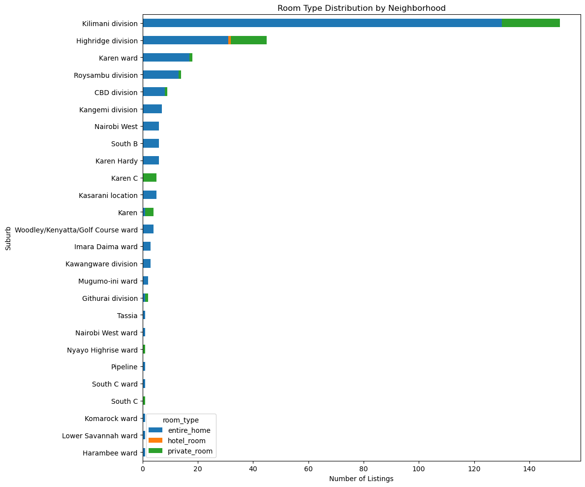 room distribution by suburb
Kilimani division overwhelmingly dominates the market, with the highest number of listings by a wide margin.
Highridge division follows as a distant second.
All other neighborhoods have relatively low listing density, many with fewer than 10 listings.
Insight: Airbnb supply in Nairobi is highly concentrated in a few prime neighborhoods rather than evenly distributed.
Entire homes make up the majority of listings in almost every suburb.
This dominance is most pronounced in Kilimani and Highridge, indicating strong demand for full-unit stays in these areas.
Interpretation: These neighborhoods likely attract:
Longer stays
Families, business travelers, or groups
Guests prioritizing privacy and space
Private rooms appear mainly in:
Kilimani
Highridge
Karen-related areas
Their presence is limited elsewhere.
Interpretation: Private rooms serve as a price-sensitive alternative in high-demand areas but are not a primary offering city-wide.
Insight: Airbnb supply in this dataset is driven by individual hosts and residential properties, not traditional hospitality players.
Karen ward shows lower volume but a mix that leans toward entire homes, consistent with its low-density, high-end residential profile.
Peripheral neighborhoods show minimal diversification, often only one room type.
area_revenue = (
    df
    .groupby('suburb')
    .agg(
        avg_annual_revenue=('revenue_per_year', 'mean'),
        avg_nightly_rate=('avg_rate_per_year', 'mean'),
        avg_occupancy=('annual_occupancy', 'mean'),
        listings_count=('listing_id', 'count')
    )
    .sort_values('avg_annual_revenue', ascending=False)
    .round(2)
)

area_revenue.head(10)
| avg_annual_revenue | avg_nightly_rate | avg_occupancy | listings_count | |
|---|---|---|---|---|
| suburb | ||||
| Karen ward | 1962535.22 | 17108.63 | 36.13 | 18 |
| Karen | 811678.25 | 8606.50 | 35.85 | 4 |
| Nairobi West ward | 712218.00 | 5552.50 | 37.60 | 1 |
| Tassia | 702593.00 | 7173.10 | 35.40 | 1 |
| Kangemi division | 661358.00 | 5242.46 | 21.89 | 7 |
| Karen Hardy | 648590.50 | 10907.72 | 18.00 | 6 |
| Kilimani division | 521143.23 | 7002.30 | 24.41 | 151 |
| Highridge division | 509475.96 | 8471.39 | 23.61 | 45 |
| Harambee ward | 502857.00 | 4460.60 | 34.40 | 1 |
| Lower Savannah ward | 471464.00 | 37484.90 | 6.50 | 1 |
area_revenue.head(10)['avg_annual_revenue'] \
.sort_values() \
.plot(kind='barh', figsize=(10, 6))
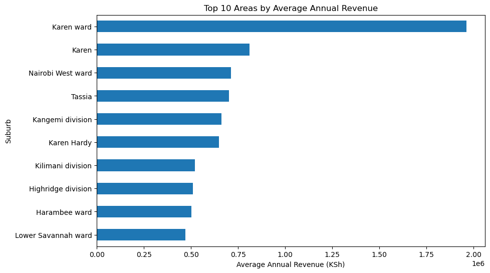
plt.title("Top 10 Areas by Average Annual Revenue")
plt.xlabel("Average Annual Revenue (KSh)")
plt.ylabel("Suburb")
plt.show()
 room distribution by suburb
Performance: Karen Ward is the undisputed market leader, generating nearly KSh 2,000,000 annually—more than double the next highest contender.
The Strategy: This dominance is driven by high Average Daily Rates (ADR) rather than sheer volume. These listings (villas, large homes) cater to the “Long Stay” market (diplomats, expats) where a single booking can secure months of revenue.
Verdict: High entry cost, but unrivaled revenue per booking.
Performance: Surprisingly, lower-middle-income areas like Nairobi West (~KSh 700k) and Tassia (~KSh 680k) significantly outperform premium hubs.
The Strategy: These areas thrive on a Volume/Occupancy model. With lower nightly rates but consistent local demand (traders, short-term work stays), they avoid the “vacancy gaps” that plague seasonal tourist spots.
Verdict: Lower entry cost with higher yield efficiency.
Performance: despite being the most famous rental hubs, Kilimani and Highridge appear in the bottom half of the top 10 (averaging ~KSh 500k).
The Strategy: These areas suffer from Oversupply. The sheer number of apartments creates fierce price competition, diluting the average revenue per host. While top-tier units earn well, the “average” unit struggles to match the returns of less saturated areas.
Verdict: High demand is offset by extreme competition; success here requires a standout product.
# Define high-revenue threshold
high_revenue_threshold = df['revenue_per_year'].quantile(0.75)

df['high_revenue'] = (
    df['revenue_per_year'] >= high_revenue_threshold
)# Create amenities count
df['amenities_count'] = (
df['amenities']
.fillna('')
.apply(lambda x: len(str(x).split(',')))
)
amenities_vs_revenue = (
    df
    .groupby('high_revenue')['amenities_count']
    .agg(['mean', 'median', 'min', 'max', 'count'])
    .round(1)
)

amenities_vs_revenue
| mean | median | min | max | count | |
|---|---|---|---|---|---|
| high_revenue | |||||
| False | 34.8 | 33.0 | 11 | 78 | 225 |
| True | 38.2 | 37.0 | 14 | 76 | 75 |
sns.boxplot(
data=df,
x='high_revenue',
y='amenities_count'
)
plt.xticks([0, 1], ['Lower Revenue', 'High Revenue'])
plt.title("Amenities Count vs Revenue Tier")
plt.ylabel("Number of Amenities")
plt.xlabel("")
plt.show()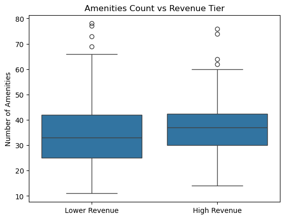 amenities and the revenue they attract
From the box plot, high-revenue listings typically have about 35–40 amenities.
More precisely:
The median (the line inside the box) is around 36–37 amenities
Most high-revenue listings (the interquartile range) fall roughly between 30 and 42 amenities
So a “typical” high-revenue listing offers mid-to-high 30s in amenities, slightly more than lower-revenue listings.
df['listing_name_length'] = (
    df['listing_name']
    .fillna('')
    .str.len()
)
correlation = df['listing_name_length'].corr(
    df['reserved_days_in_year']
)

correlationnp.float64(0.10077962524781812)df['name_length_bin'] = pd.qcut(
df['listing_name_length'],
q=4,
labels=['Short', 'Medium', 'Long', 'Very Long']
)
df.groupby('name_length_bin')['reserved_days_in_year'].mean().sort_values(ascending=False)
/tmp/ipykernel_54075/1443461262.py:7: FutureWarning: The default of observed=False is deprecated and will be changed to True in a future version of pandas. Pass observed=False to retain current behavior or observed=True to adopt the future default and silence this warning.
  df.groupby('name_length_bin')['reserved_days_in_year'].mean().sort_values(ascending=False)


name_length_bin
Very Long    86.812500
Long         73.047059
Short        70.526316
Medium       65.720000
Name: reserved_days_in_year, dtype: float64sns.scatterplot(
data=df,
x='listing_name_length',
y='reserved_days_in_year',
alpha=0.6
)
sns.regplot(
data=df,
x='listing_name_length',
y='reserved_days_in_year',
scatter=False,
color='red'
)
plt.title("Listing Name Length vs Booked Nights per Year")
plt.xlabel("Listing Name Length (characters)")
plt.ylabel("Booked Nights per Year")
plt.show()
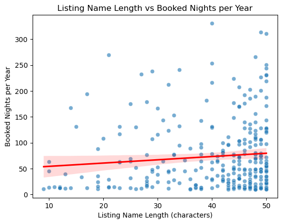 Correlation between listing name and booked nights per year
The red regression line slopes slightly upward, indicating a weak positive relationship between listing name length and booked nights per year.
This means that, on average, listings with longer names tend to receive slightly more bookings, but the effect is not strong.
The points are widely scattered around the line.
This high dispersion shows that listing name length alone explains very little of the variation in bookings.
Many listings with long names still have low bookings, and some short names perform very well.
Conclusion: The relationship exists, but it is weak.
Longer names likely help by:
Including keywords (location, amenities, “near CBD”, “luxury”, etc.)
Improving clarity and search visibility
However, bookings are far more influenced by:
Location
Price
Reviews
Amenities
Professional management
df| listing_id | listing_name | listing_type | room_type | cover_photo_url | photos_count | minimum_nights | cancellation_policy | professional_management | registration | ... | price_range | neighbourhood | suburb | county | city | postcode | high_revenue | amenities_count | listing_name_length | name_length_bin | |
|---|---|---|---|---|---|---|---|---|---|---|---|---|---|---|---|---|---|---|---|---|---|
| 0 | 75683 | Kiloranhouse Apt Prime Bedroom | Private room in home | private_room | https://a0.muscache.com/im/pictures/5499026/ef... | 13 | 2 | Moderate | False | False | ... | Mid-range (5-10k) | Kilimani ward | Kilimani division | None | Nairobi | 30728 | False | 42 | 30 | Short |
| 1 | 471581 | Located In a Serene Environment | Entire cottage | entire_home | https://a0.muscache.com/im/pictures/6434524/bc... | 37 | 2 | Moderate | False | False | ... | Mid-range (5-10k) | Roysambu location | Roysambu division | None | Nairobi | 31224 | True | 24 | 31 | Short |
| 2 | 906958 | Makena's Place Karen - Flamingo Room | Private room in cottage | private_room | https://a0.muscache.com/im/pictures/68ecc57f-d... | 29 | 1 | Firm | False | False | ... | Mid-range (5-10k) | None | Karen | None | Nairobi | 00505 | False | 30 | 36 | Medium |
| 3 | 1023556 | Guesthouse Near Nairobi National Park & Airport | Entire guesthouse | entire_home | https://a0.muscache.com/im/pictures/ddd8badc-1... | 20 | 1 | Flexible | False | False | ... | Budget (0-5k) | None | Mugumo-ini ward | None | Nairobi | 00517 | False | 33 | 47 | Long |
| 4 | 1237886 | Hob House | Room in bed and breakfast | hotel_room | https://a0.muscache.com/im/pictures/cbdab7e1-f... | 8 | 1 | Flexible | True | False | ... | Luxury (15k+) | Highridge location | Highridge division | None | Nairobi | 11403 | False | 42 | 9 | Short |
| ... | ... | ... | ... | ... | ... | ... | ... | ... | ... | ... | ... | ... | ... | ... | ... | ... | ... | ... | ... | ... | ... |
| 295 | 42123446 | Mvuli Luxury Suites | Entire rental unit | entire_home | https://a0.muscache.com/im/pictures/238557fd-c... | 24 | 1 | Firm | False | False | ... | Budget (0-5k) | Ngara location | CBD division | None | Nairobi | 45046 | False | 32 | 19 | Short |
| 296 | 42139551 | Modern 1BR | King Bed | Fast Wi-Fi | Near CBD | Entire condo | entire_home | https://a0.muscache.com/im/pictures/a10f889a-4... | 27 | 1 | Flexible | False | False | ... | Mid-range (5-10k) | Kilimani ward | Kilimani division | None | Nairobi | 30728 | False | 53 | 45 | Long |
| 297 | 42187559 | Cosy & Airy Studio with Balcony WI-FI and Netflix | Tiny home | entire_home | https://a0.muscache.com/im/pictures/miso/Hosti... | 43 | 1 | Moderate | True | False | ... | Budget (0-5k) | Kangemi location | Kangemi division | None | Nairobi | 29326 | False | 60 | 49 | Very Long |
| 298 | 42207619 | Kazuri Ivy Serene & Spacious Nairobi Apartment | Entire rental unit | entire_home | https://a0.muscache.com/im/pictures/hosting/Ho... | 19 | 2 | Moderate | False | False | ... | Budget (0-5k) | Ngara location | CBD division | None | Nairobi | 45046 | False | 20 | 46 | Long |
| 299 | 42223689 | Airy & Light-Filled: Indoor-Outdoor Home-Stay | Private room in rental unit | private_room | https://a0.muscache.com/im/pictures/fd146f8e-5... | 17 | 2 | Moderate | False | False | ... | Budget (0-5k) | Kileleshwa location | Kilimani division | None | Nairobi | 54102 | False | 55 | 45 | Long |
300 rows × 52 columns
price_bins = [0, 3000, 6000, 10000, 15000, df['avg_rate_per_year'].max()]
price_labels = [
    'Low (0–3k)',
    'Lower-Mid (3k–6k)',
    'Mid (6k–10k)',
    'Upper-Mid (10k–15k)',
    'Premium (15k+)'
]

df['price_band'] = pd.cut(
    df['avg_rate_per_year'],
    bins=price_bins,
    labels=price_labels,
    include_lowest=True
)
market_summary = (
    df.groupby(['room_type', 'price_band'])
      .agg(
          listings_count=('listing_id', 'count'),
          avg_occupancy=('annual_occupancy', 'mean'),
          avg_revenue=('revenue_per_year', 'mean')
      )
      .reset_index()
)
/tmp/ipykernel_54075/1390846018.py:2: FutureWarning: The default of observed=False is deprecated and will be changed to True in a future version of pandas. Pass observed=False to retain current behavior or observed=True to adopt the future default and silence this warning.
df.groupby(['room_type', 'price_band'])supply_threshold = market_summary['listings_count'].median()
occupancy_threshold = market_summary['avg_occupancy'].median()
revenue_threshold = market_summary['avg_revenue'].median()
market_summary['underrepresented'] = (
    (market_summary['listings_count'] < supply_threshold) &
    (
        (market_summary['avg_occupancy'] > occupancy_threshold) |
        (market_summary['avg_revenue'] > revenue_threshold)
    )
)

underrepresented_segments = market_summary[
    market_summary['underrepresented']
].sort_values(['avg_occupancy', 'avg_revenue'], ascending=False)

underrepresented_segments
| room_type | price_band | listings_count | avg_occupancy | avg_revenue | underrepresented | |
|---|---|---|---|---|---|---|
| 14 | private_room | Premium (15k+) | 5 | 5.32 | 363316.2 | True |
supply_by_price = (
    df.groupby('price_band')
      .agg(
          listings_count=('listing_id', 'count'),
          avg_price=('avg_rate_per_year', 'mean')
      )
      .reset_index()
)
/tmp/ipykernel_54075/1042693843.py:2: FutureWarning: The default of observed=False is deprecated and will be changed to True in a future version of pandas. Pass observed=False to retain current behavior or observed=True to adopt the future default and silence this warning.
df.groupby('price_band')performance_by_price = (
df.groupby('price_band')
.agg(
avg_occupancy=('annual_occupancy', 'mean'),
avg_revenue=('revenue_per_year', 'mean')
)
.reset_index()
)
/tmp/ipykernel_54075/2880606656.py:2: FutureWarning: The default of observed=False is deprecated and will be changed to True in a future version of pandas. Pass observed=False to retain current behavior or observed=True to adopt the future default and silence this warning.
df.groupby('price_band')price_gap_analysis = supply_by_price.merge(
performance_by_price,
on='price_band'
)
price_gap_analysis.sort_values('listings_count')
| price_band | listings_count | avg_price | avg_occupancy | avg_revenue | |
|---|---|---|---|---|---|
| 4 | Premium (15k+) | 21 | 23956.961905 | 23.223810 | 1.874120e+06 |
| 3 | Upper-Mid (10k–15k) | 30 | 11954.396667 | 22.013333 | 8.627922e+05 |
| 0 | Low (0–3k) | 41 | 2346.365854 | 23.697561 | 1.668768e+05 |
| 1 | Lower-Mid (3k–6k) | 97 | 4616.963918 | 23.797938 | 3.463240e+05 |
| 2 | Mid (6k–10k) | 111 | 7618.214414 | 23.310811 | 5.501002e+05 |
price_gap_analysis['potential_gap'] = (
    (price_gap_analysis['listings_count'] < price_gap_analysis['listings_count'].median()) &
    (price_gap_analysis['avg_occupancy'] > price_gap_analysis['avg_occupancy'].median())
)

price_gap_analysis
| price_band | listings_count | avg_price | avg_occupancy | avg_revenue | potential_gap | |
|---|---|---|---|---|---|---|
| 0 | Low (0–3k) | 41 | 2346.365854 | 23.697561 | 1.668768e+05 | False |
| 1 | Lower-Mid (3k–6k) | 97 | 4616.963918 | 23.797938 | 3.463240e+05 | False |
| 2 | Mid (6k–10k) | 111 | 7618.214414 | 23.310811 | 5.501002e+05 | False |
| 3 | Upper-Mid (10k–15k) | 30 | 11954.396667 | 22.013333 | 8.627922e+05 | False |
| 4 | Premium (15k+) | 21 | 23956.961905 | 23.223810 | 1.874120e+06 | False |
Revenue trend analysis typically requires time-series data. As this dataset provides a snapshot of listing performance rather than longitudinal observations, it does not support direct analysis of declining or increasing revenue trends by listing type. Instead, the analysis focuses on comparing current revenue performance across listing categories.