Crop Recommendation Engine
Prepared for: the client
Submission: Jupyter Notebook, Cleaned Dataset, PDF Report, README
Executive Summary
This report includes details on the build, evaluation, and findings of a baseline crop recommendation engine for the project using the Kaggle Crop Recommendation Dataset. The primary objective of this project was to leverage machine learning to provide data-driven insights that assist in selecting the most suitable crops based on environmental and soil conditions.
The dataset required no cleaning; the data-cleaning step was largely a verification exercise to ensure structural integrity and the absence of missing values. This allowed for an immediate transition into deeper analysis and feature transformation.
Three engineered features (NPK Score, Climate Sustainability Index, and Categorical Soil Suitability) were derived from existing features in the Feature Engineering Phase to better capture the complex relationships between soil nutrients and climate stability.
I decided to use a classifier model KNN classifier inside a single Scikit-Learn Pipeline, trained on an 80/20 stratified split with all preprocessing statistics learned only from the training partition. This methodological approach ensures that the model evaluation is unbiased and representative of real-world performance. On the held-out test set, the model reached 97.50% Top-1 and 99.77% Top-3 accuracy, confirmed as stable by 5-fold cross-validation (97.27% mean, 0.66% standard deviation). The trained pipeline was serialized to disk and verified to reload and predict correctly, ensuring it is production-ready for deployment in agricultural decision-support systems.
Introduction
The project aims to deliver precise crop recommendations by analyzing environmental and historical data. This
assessment details an end-to-end pipeline covering data sourcing, cleaning, exploratory analysis, feature engineering, and engine implementation, including an LLM-based qualitative analysis.
Following the data science lifecycle, this report relies on analysis.ipynb as the sole source of truth for all metrics.
Data Preparation
The dataset aligns with three of the project’s recommendation pillars: soil properties (N, P, K, pH), climate conditions, and crop performance. Lacking explicit location data, climate variables serve as a geographical proxy.
Validation confirmed zero missing values or duplicate rows, with all readings within valid ranges. Outlier screening was performed per crop via IQR bounds to avoid misclassifying legitimate crop-specific extremes. No outliers were found, and the final set was exported to cleaned_crop_data.csv.
Exploratory Data Analysis
Standard deviation analysis identifies Potassium (50.65 ppm) and rainfall (54.96 mm) as the most volatile metrics, while pH (0.77) is the most stable. This stability reflects the similar soil acidity tolerances shared by the 22 analyzed crop species, despite their varying nutrient and water needs.
The correlation matrix confirms these variables are largely independent, with most coefficients (|r|) below 0.25. This indicates the seven predictors offer complementary data for the engine. Although Phosphorus and Potassium show a moderate correlation (r = 0.74), both are retained as they provide distinct agronomic signals.
Numeric Feature Correlation Matrix
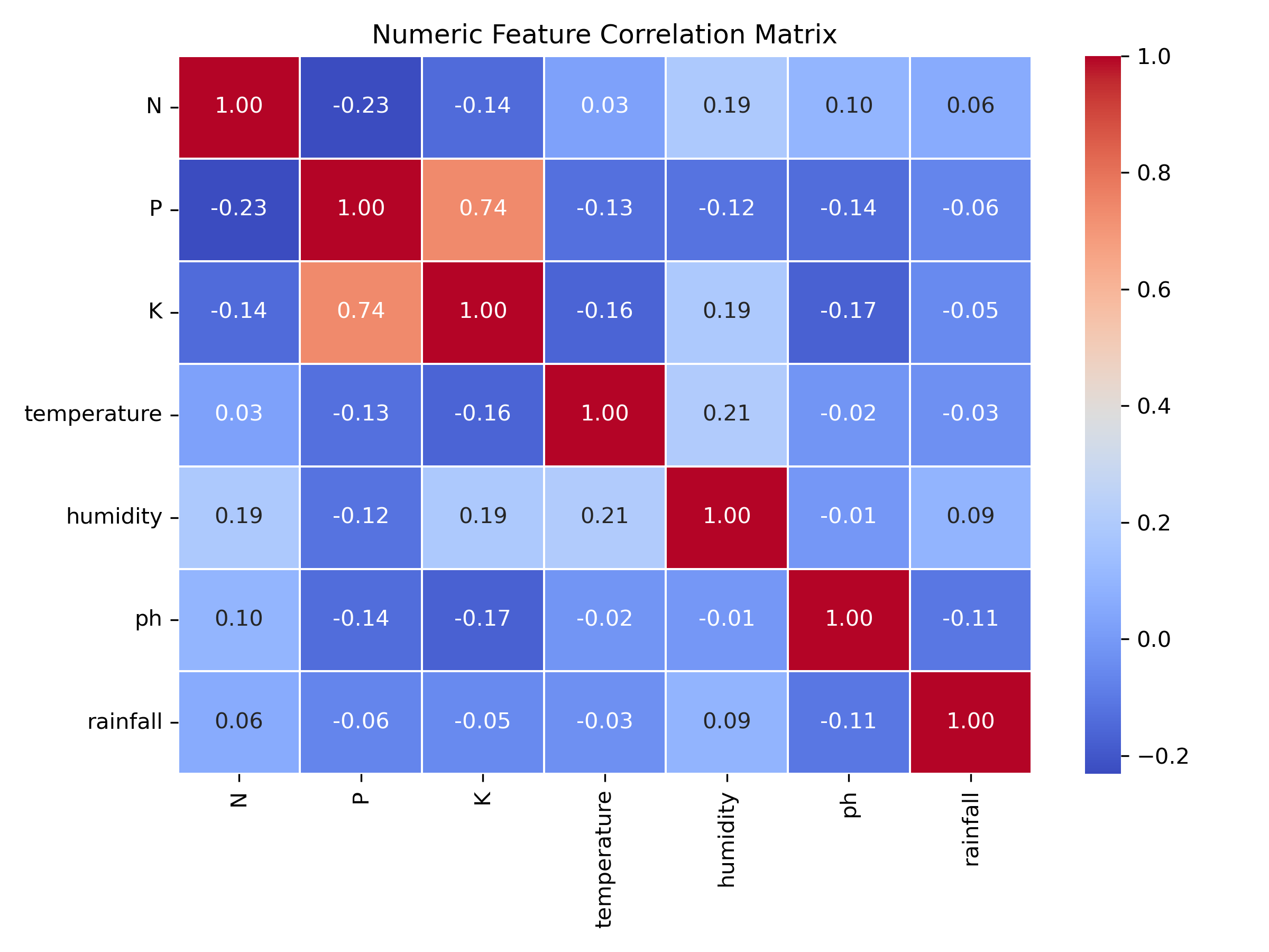 Figure 1. Correlation matrix across the seven numeric features.
Why it matters: Because the predictors mostly carry independent signals, the model benefits from using all seven raw features together rather than a reduced subset.
Rainfall requirements separate crops sharply: rice needs the most (median ≈ 236 mm) while muskmelon needs the least (median ≈ 22 mm) — over a tenfold difference.
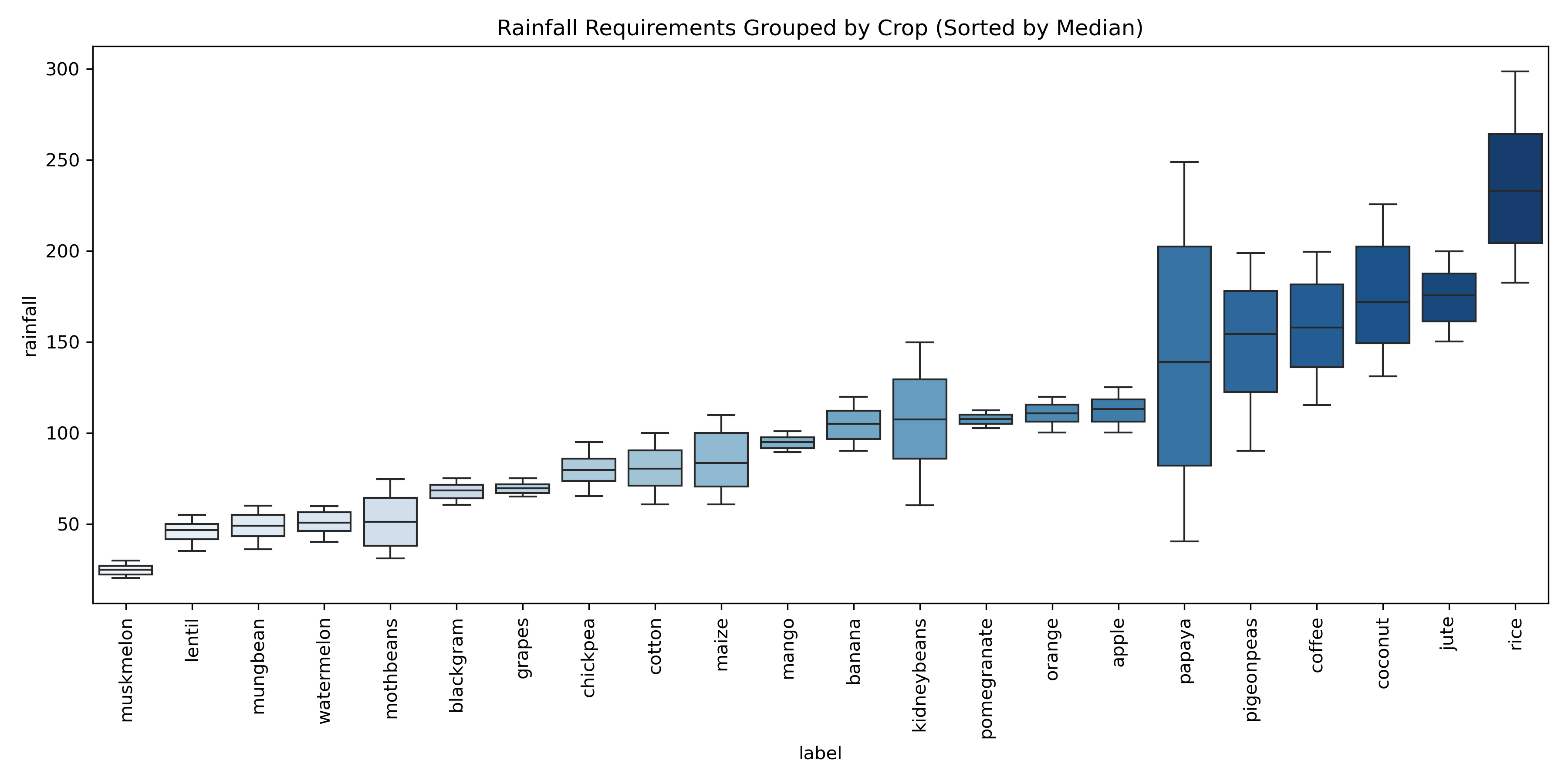 Figure 2. Rainfall distribution per crop, sorted by median.
A radar chart of min-max scaled feature means for five representative crops (rice, grapes, coffee, muskmelon, banana) provides a visual multi-dimensional fingerprint, revealing how each crop occupies a unique niche within the seven-feature environmental space. Specifically, rice presents a profile heavily skewed toward high nitrogen, humidity, and rainfall, reflecting its intensive irrigation and nutrient needs. In contrast, grapes exhibit a distinctive shape characterized by exceptionally high phosphorus and potassium levels while remaining low on the rainfall axis. Coffee appears as a more balanced, centrally located shape but with a notable lean toward higher soil acidity. Muskmelon occupies a profile defined by high humidity and temperature coupled with very low rainfall requirements, while banana profiles pair high nitrogen levels with high humidity. These distinct geometric patterns confirm that each crop is defined not by a single threshold, but by a complex, multi-feature agronomic signature.
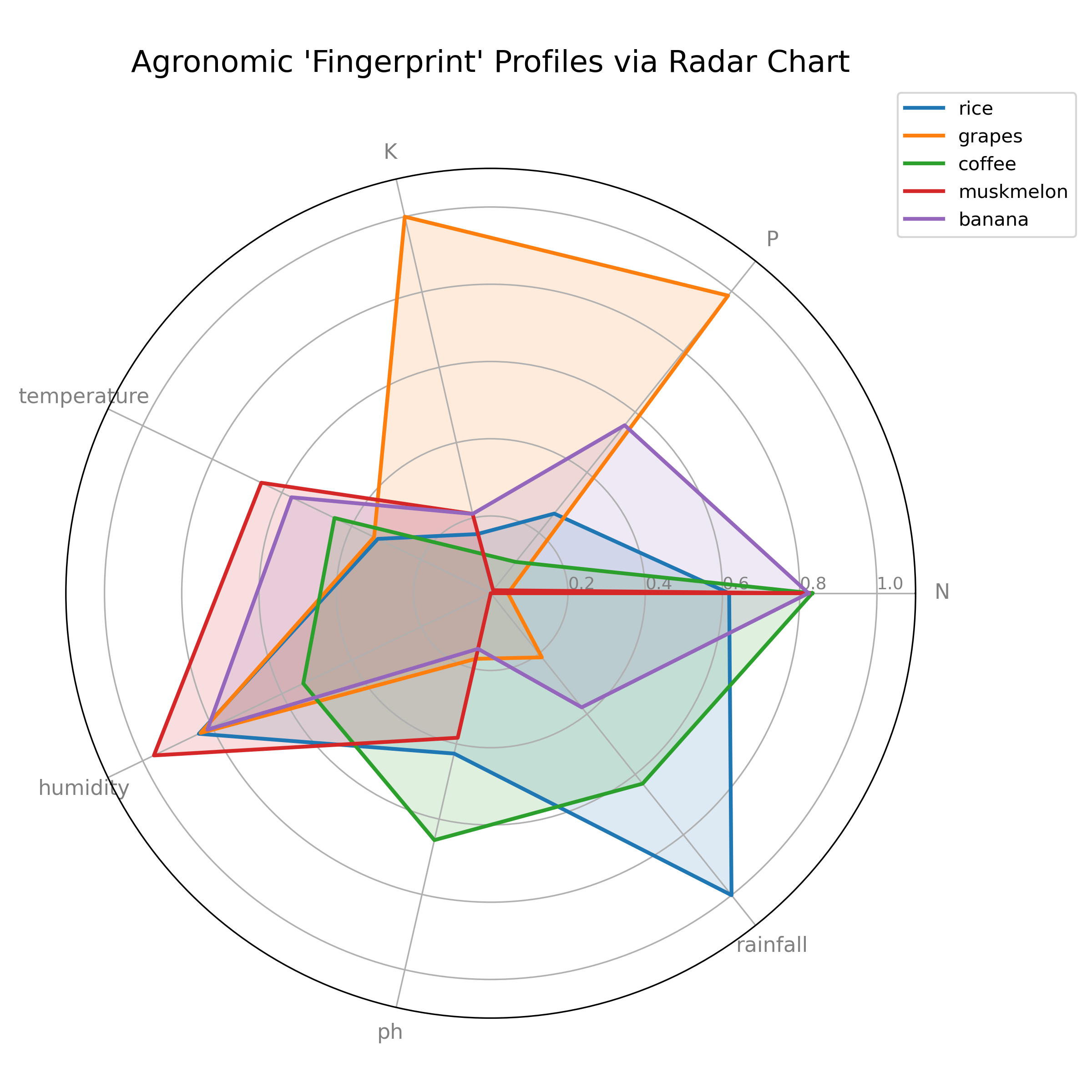 Figure 3. Multi-feature agronomic fingerprints for five representative crops.
Why it matters: No crop is defined by a single dominant feature — each has a distinct combination across all seven variables. This is the core justification for a similarity-matching model over any single-threshold rule.
Feature Engineering
To enhance the model’s predictive power, three specific features were engineered, each computable from data the project already collects, such as routine soil tests and weather readings. Two of these, the NPK Score and the Climate Suitability Index, depend on dataset-wide statistics. To ensure a robust evaluation, the cleaned data was split 80/20 (stratified) before any such statistic was computed. This methodological rigor prevents test-set information from leaking into training, ensuring that the model’s performance metrics are a true reflection of its ability to generalize to unseen agricultural data.
| Feature | Formula | Why it helps |
|---|
| NPK Score | (N_scaled + P_scaled + K_scaled) / 3 | Summarizes overall soil fertility in one value, |
| | complementing raw N/P/K. |
| Climate Suitability Index | (Z_temp + Z_humidity + Z_rainfall) / 3 | Summarizes climate fit; separates crops with similar soil |
| | but different weather needs. |
| Soil Suitability Category | Acidic <6.5 · Neutral 6.5–7.5 · Alkaline >7.5 | Converts pH into farmer-familiar soil classes without |
| | discarding the raw value. |
All three are implemented in a custom AgronomicFeatureEngineer transformer whose fit() learns statistics only from the data it receives, and whose transform() applies them, making it safe to reuse inside cross-validation folds, each of which computes its own parameters independently.
Model Development & Evaluation
Advantages of KNN over Centroid Matching
While a centroid approach simplifies each crop into a single average profile, it ignores the natural variability shown in the boxplots. This can lead to misjudgments for farmers whose conditions fall near the edges of a crop’s range. Instead, K-Nearest Neighbors (k=5, Euclidean distance) compares a farmer’s profile against individual historical observations. This method preserves variability and enables a ranked, probability-scored Top-N recommendation through predict_proba, a capability centroid matching lacks without significant modifications. KNN was thus selected for its robustness.
Pipeline Integration and Reproducibility
Feature engineering, Min-Max scaling, and the KNN classifier are integrated into a single Scikit-Learn Pipeline. Scaling is vital because Euclidean distance is sensitive to features with larger numeric ranges, such as rainfall. By encapsulating every step within the Pipeline, refitting on any new data split ensures identical transformations without manual tracking. This structure prevents data leakage and guarantees consistent reproducibility across environments.
Testing with the provided example (N=85, P=40, K=50, pH=6.5, rainfall=120 mm), the pipeline recommends jute (100% probability). The explanation layer helpfully notes that the input rainfall (120 mm) is below the typical training range (~161–191 mm), though it remains the most suitable match. Such context is invaluable for farmers evaluating these suggestions.
On the 440-row test set, the pipeline achieved 97.50% Top-1 accuracy and 99.77% Top-3 accuracy, mirroring how farmers utilize a shortlist of options. The weighted F1-score is 0.97. No specific class performed poorly; the lowest-recall categories (lentil, mothbeans, jute, and rice) were only confused with agronomically similar neighbors, as evidenced in the confusion matrix.
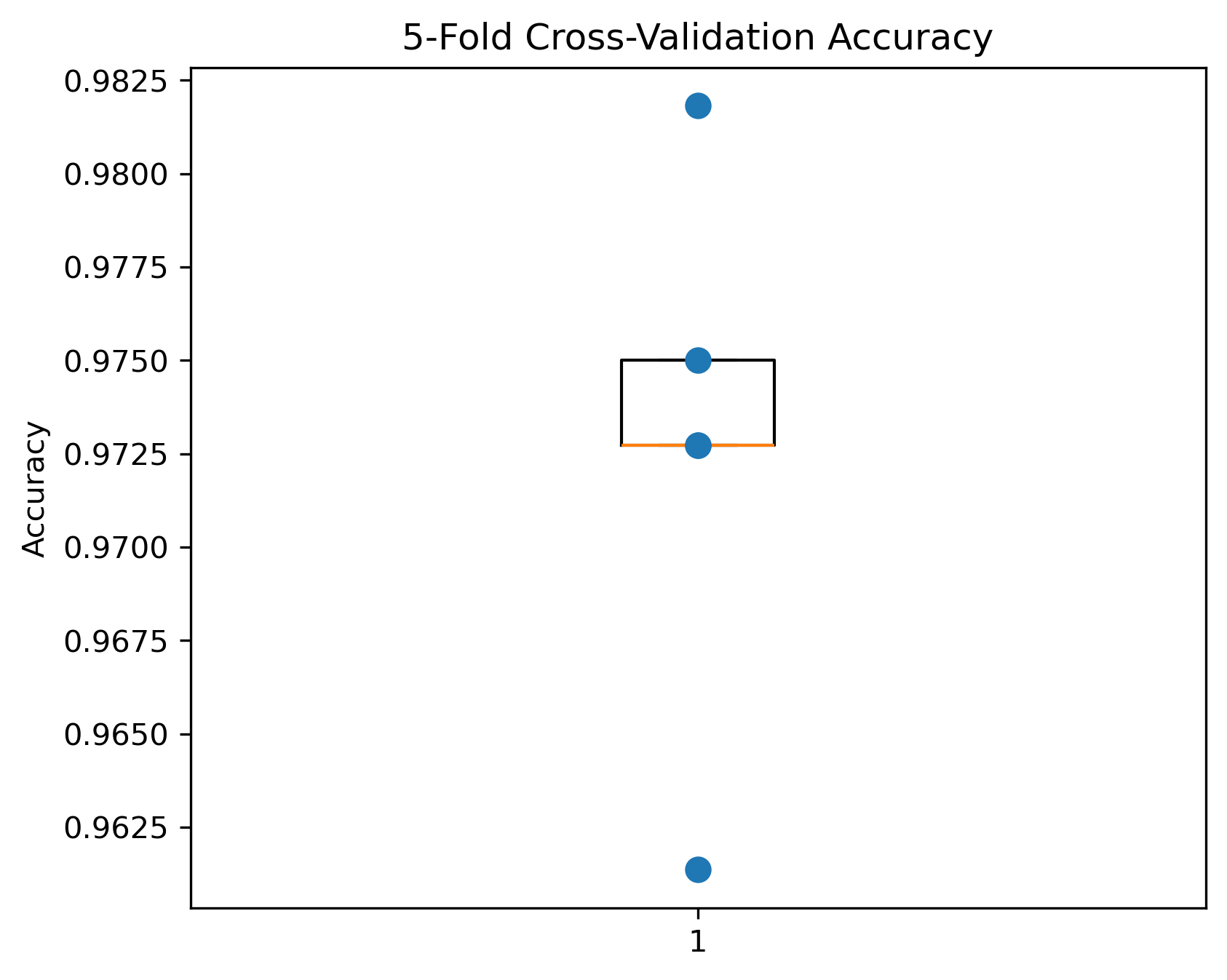 Figure 5. Accuracy across 5 stratified CV folds.
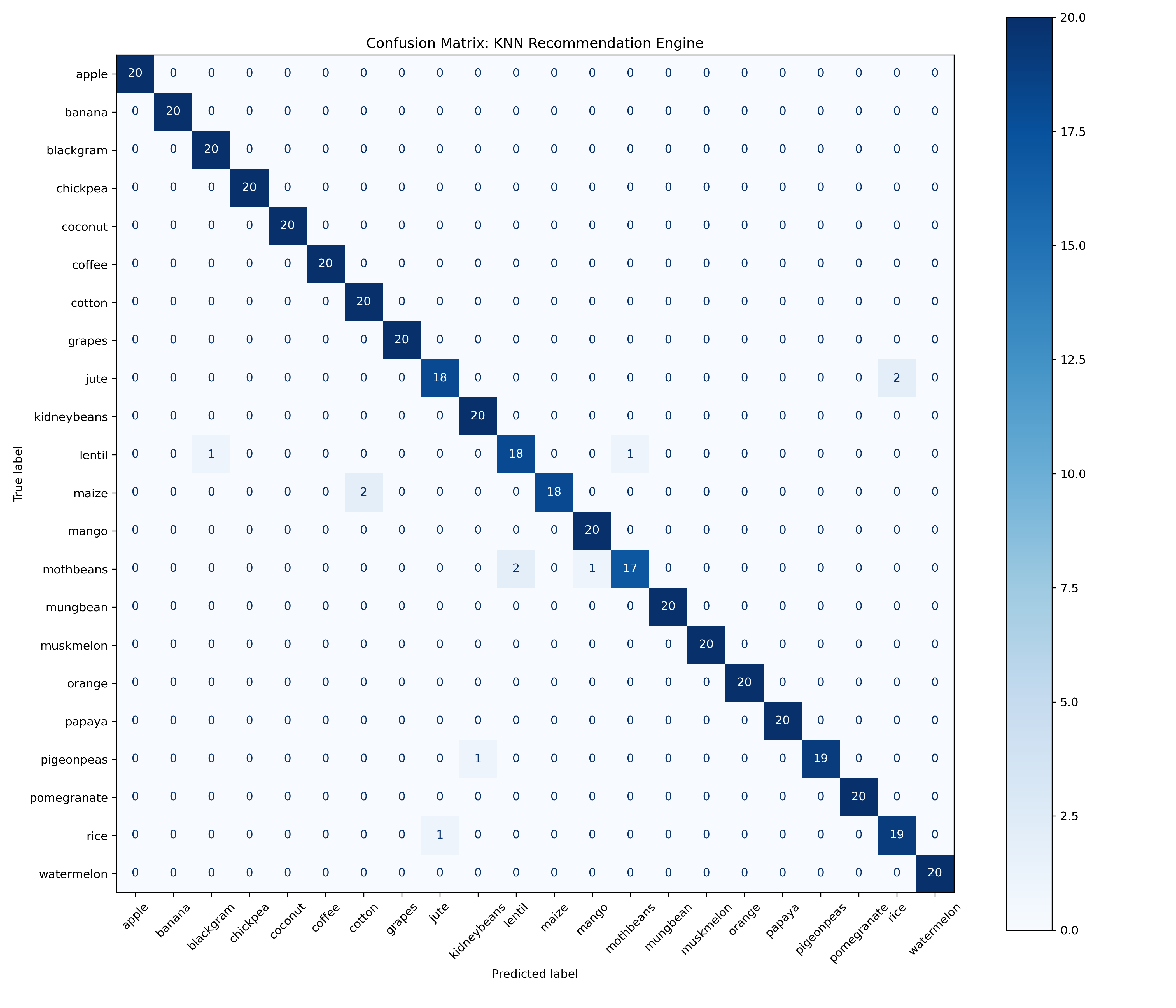 Figure 4. Confusion matrix (440-row test set, 22
classes).
Errors cluster between related pairs (rice/jute, lentil/blackgram), not random classes — a low-cost failure mode. Five-fold stratified cross-validation returned 97.27% mean accuracy with 0.66% standard deviation, confirming the single test-split result is not a lucky partition.
The entire pipeline was serialized using joblib into a portable .joblib artifact. Successful reloading and identical prediction on the worked example confirm that the system is deployment-ready, requiring no additional preprocessing code to function in production.
LLM Reflection (Bonus Task)
A zero-shot prompt to Google Gemini, outlining the dataset structure, requested predictions on crop clustering based on rainfall and NPK profiles using agronomic knowledge. Gemini hypothesized that rice would form an isolated cluster due to high rainfall/humidity, that grapes and apples would occupy a distinct high-potassium region, that legumes would cluster around low nitrogen, and that field crops like maize would exhibit heavy overlap.
The EDA confirmed the rice and grape hypotheses (Figures 2–3) and supported the field-crop overlap claim observed in the confusion matrix. The legume hypothesis required refinement: while lentil and blackgram do confuse the model, nitrogen levels alone cannot separate legumes across all 22 classes—separation requires the combination of all seven features. While Gemini successfully identified key visualizations to prioritize, it could not perform statistical calculations; consequently, all metrics in this report were independently verified against the analysis notebook.
Limitations
-
Missing Location Data: Climate variables function only as proxies for the project’s fourth recommendation pillar.
-
Idealized Data Quality: The absence of missing, duplicate, or outlier data is unrepresentative of live field sensors; production systems will require robust imputation logic.
-
Untuned Hyperparameters: A K-value of 5 was used as a baseline per the brief’s guidelines, rather than an optimized grid-searched value.
-
Limited Stability Scope: Cross-validation validates performance across random data splits, but does not guarantee stability across unseen regions or seasons.
Conclusion
The delivered pipeline establishes an end-to-end process from raw data to a serialized, verified recommendation model, ensuring all leakage-sensitive operations remain isolated within the training partition. The model achieves 97.50% Top-1 and 99.77% Top-3 accuracy on held-out test data, with performance confirmed stable by cross-validation. Furthermore, model errors remain confined to agronomically similar crops, a low-cost failure mode. The logical next step for the project is to integrate this pipeline with geographically tagged, real-time sensor data and develop the necessary imputation logic for production deployment.
Note
The accompanying notebook is part of a complete project and relies on supporting source files, serialized model artifacts, and the expected repository structure. The full project, setup instructions, and documentation are available at:
GitHub: https://github.com/Kobeyvines/Crop_Recommendation
README.MD:
The repository README includes instructions for installing dependencies, recreating the excluded data/ directory (managed locally using Git LFS/DVC), downloading the dataset, and running the project successfully.